fastai
fastai
A deep learning library
for fast implementation
& research
for fast implementation
& research
Marie-Hélène Burle
Marie-Hélène Burle
April 14, 2021

WestGrid Training Modules 2021

https://wgtm21.netlify.app/
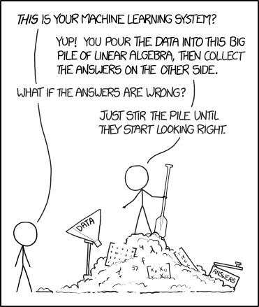
Machine learning
Dominant approach:
History
1943: Warren McCulloch & Walter Pitts—mathematical model of artificial neuron.
1961: Frank Rosenblatt—perceptron.
1961: Arthur Samuel’s checkers program.
1986: James McClelland, David Rumelhart & PDP Research Group—book: “Parallel Distributed Processing”.
Neurons
Schematic from <a href="https://commons.wikimedia.org/w/index.php?curid=1474927" target="_blank">Dhp1080, Wikipedia</a>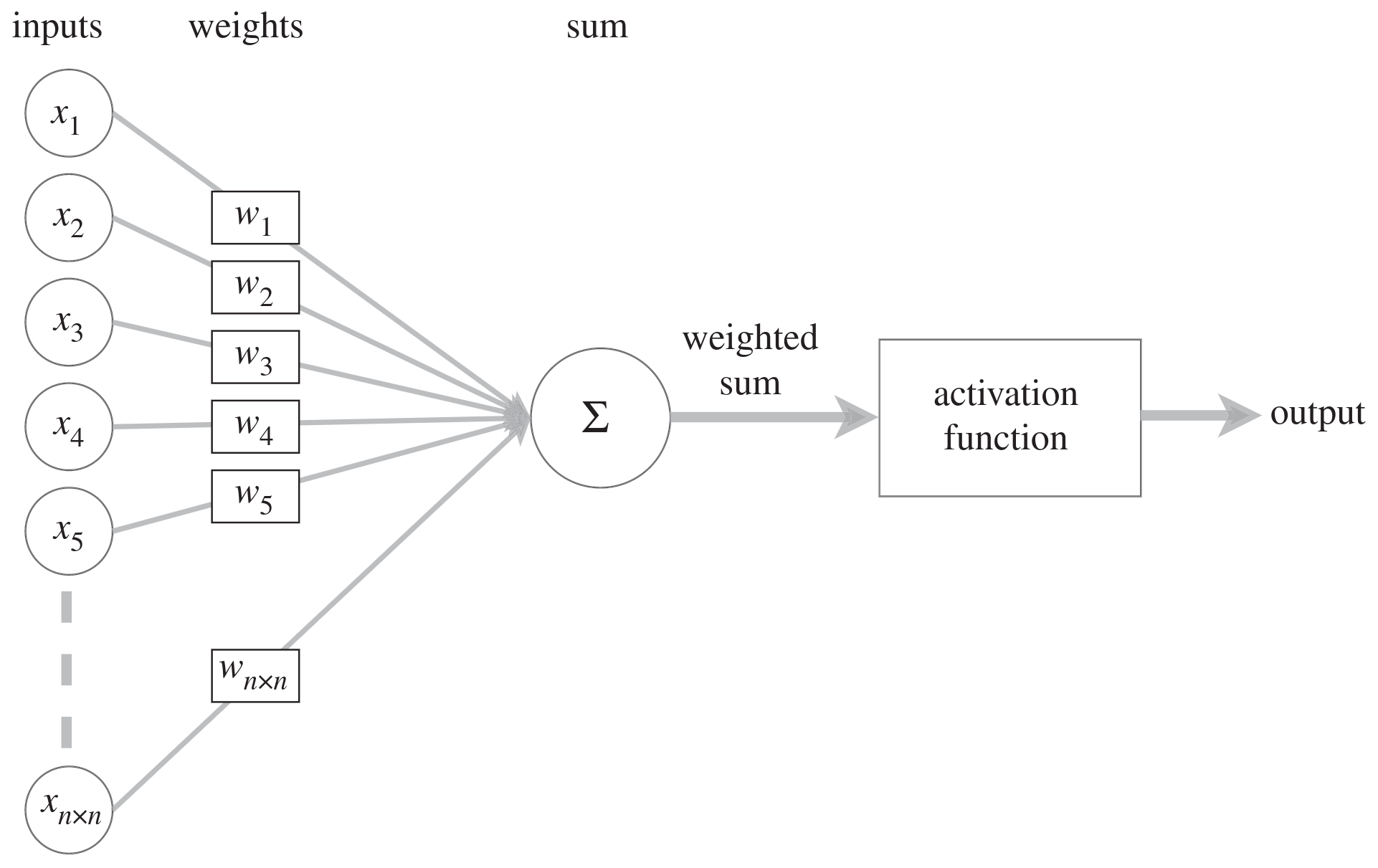
Modified from <a href="https://royalsocietypublishing.org/doi/10.1098/rsta.2019.0163" target="_blank">O.C. Akgun & J. Mei 2019</a>Neural networks
A NN is a parameterized function which can, in theory, solve any problem to any level of accuracy.
The learning process is the mapping of input data to output data (in a training set) through the adjustment of the parameters.
Neural networks

Image by <a href="https://news.berkeley.edu/2020/03/19/high-speed-microscope-captures-fleeting-brain-signals/" target="_blank">Na Ji, UC Berkeley</a>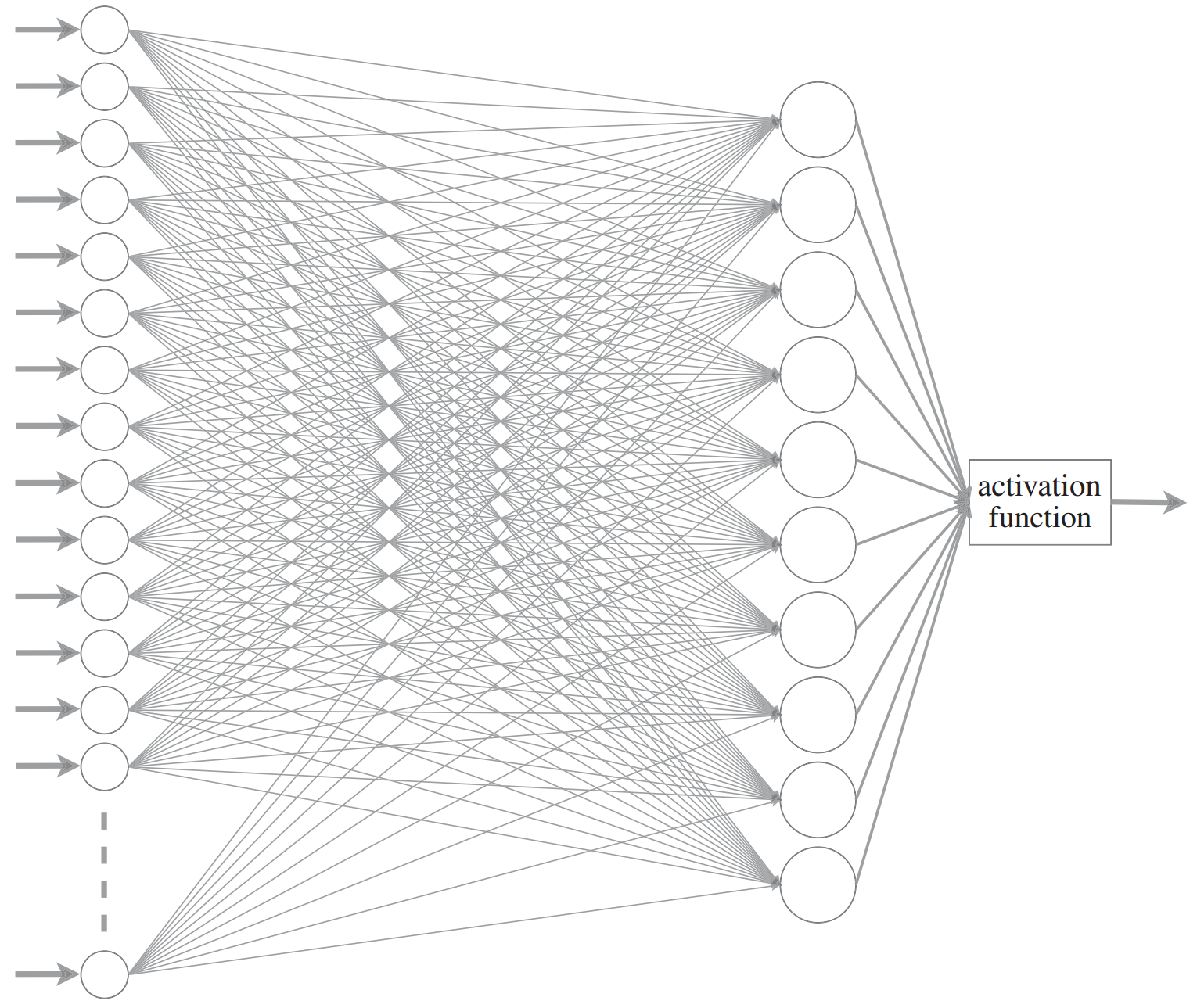
Modified from <a href="https://royalsocietypublishing.org/doi/10.1098/rsta.2019.0163" target="_blank">O.C. Akgun & J. Mei 2019</a>Neural networks
Single layer of artificial neurons → Unable to learn even some of the simple mathematical functions (Marvin Minsky & Seymour Papert).
Two layers → Theoretically can approximate any math model, but in practice very slow.
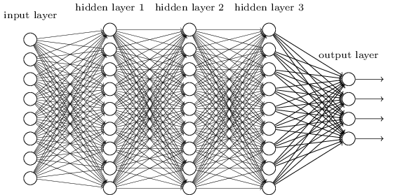
More layers → Deeper networks
Neural networks
Single layer of artificial neurons → Unable to learn even some of the simple mathematical functions (Marvin Minsky & Seymour Papert).
Two layers → Theoretically can approximate any math model, but in practice very slow.
More layers → Deeper networks → deep learning.
Types of NN
Fully-connected, feedforward, single-layer NN

Fully-connected, feedforward, deep NN
Convolutional neural network (CNN)
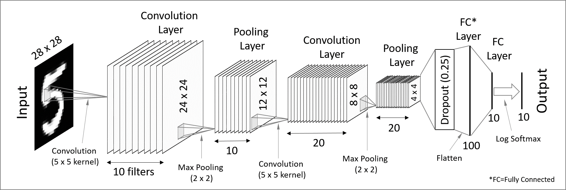
Used for spatially structured data.
Convolution layers → each neuron receives input only from a subarea of the previous layer.
Pooling → combines the outputs of neurons in a subarea to reduce the data dimensions.
Not fully connected.
Recurrent neural network (RNN)
Used for chain structured data (e.g. text).
Not feedforward.
General principles
Building a model

First, we need an architecture (size, depth, types of layers, etc.).
This is set before training and does not change.
Building a model

A model also comprises parameters.
Those are set to some initial values, but will change during training.
Training a model

To train the model, we need labelled data in the form of input/output pairs.
Training a model

Inputs and parameters are fed to the architecture.
Training a model

We get predictions as outputs.
Training a model

A metric (e.g. error rate) compares predictions and labels and is a measure of model performance.
Training a model
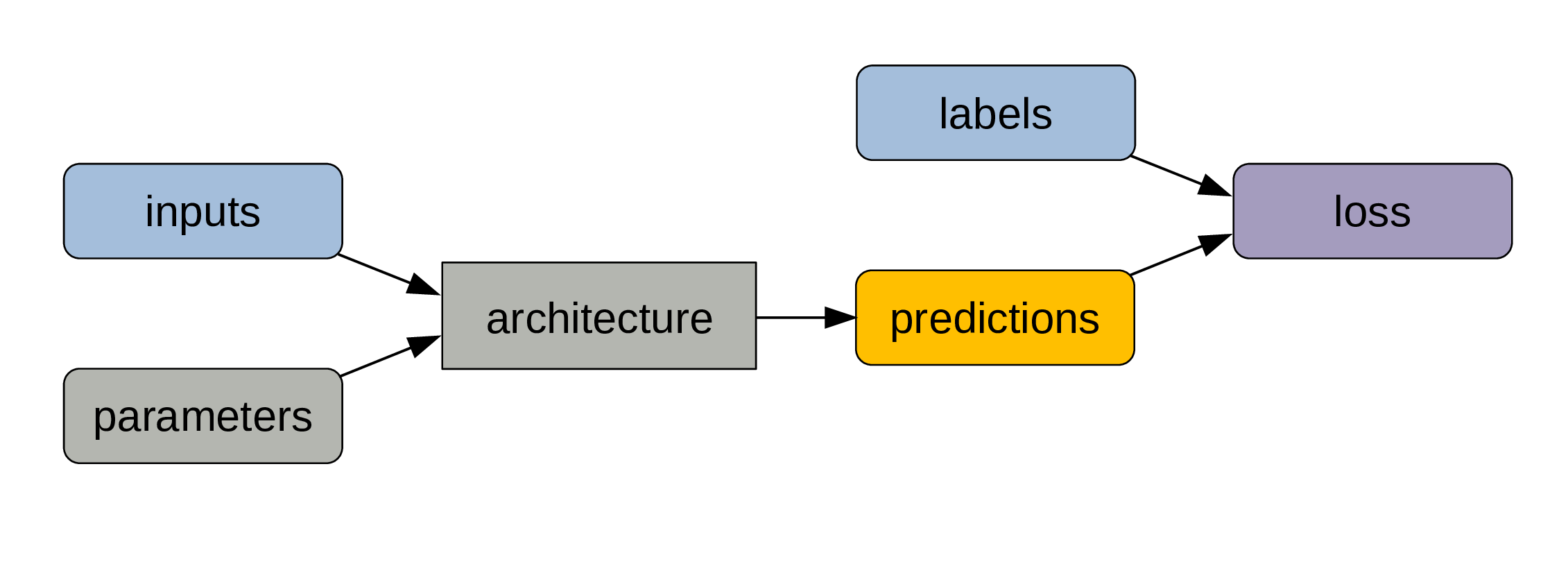
Because it is not always sensitive enough to changes in parameter values, we compute a loss function …
Training a model

… which allows to adjust the parameters slightly through backpropagation.
This cycle gets repeated for a number of steps.
Using a model

At the end of the training process, what matters is the combination of architecture and trained parameters.
Using a model
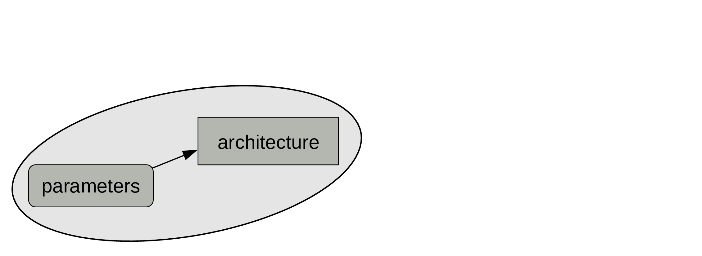
That’s what constitute a model.
Using a model

A model can be considered as a regular program …
Using a model
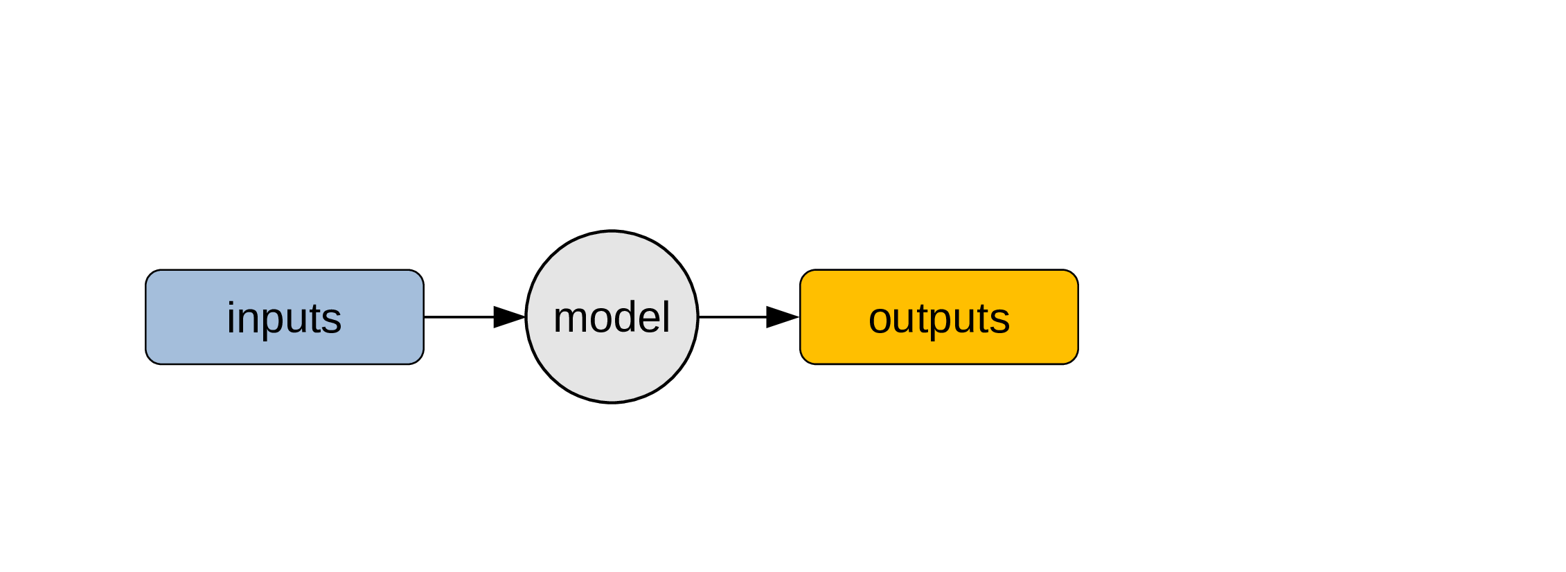
… and be used to obtain outputs from inputs.
fastai
What is fastai?
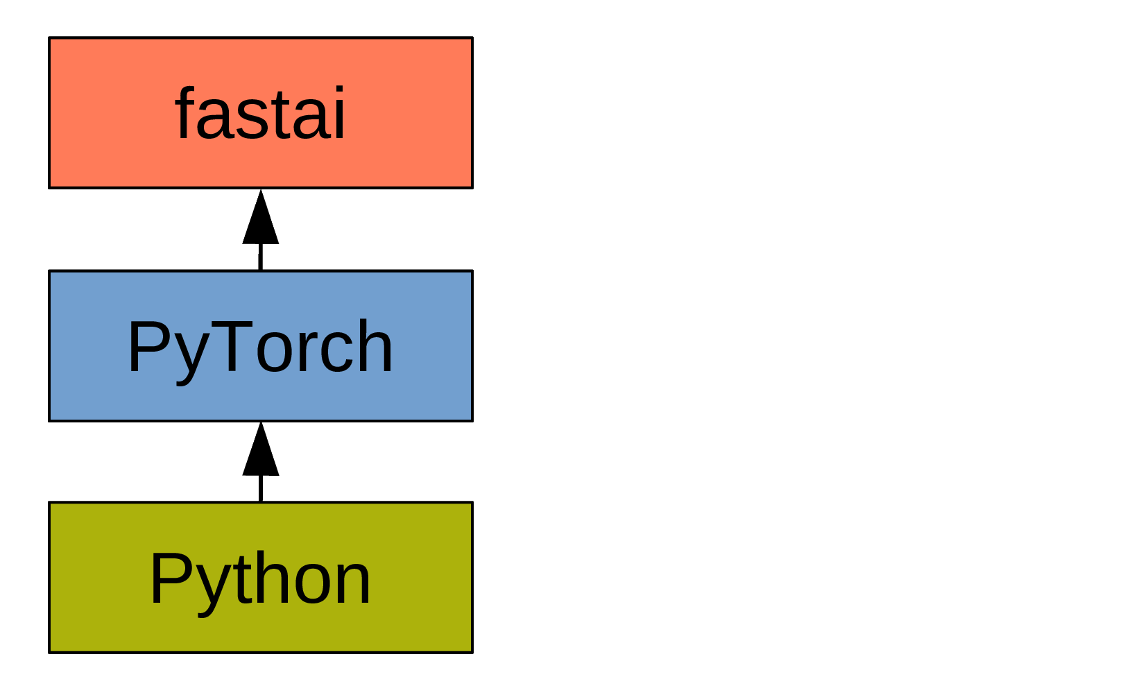
What is fastai?
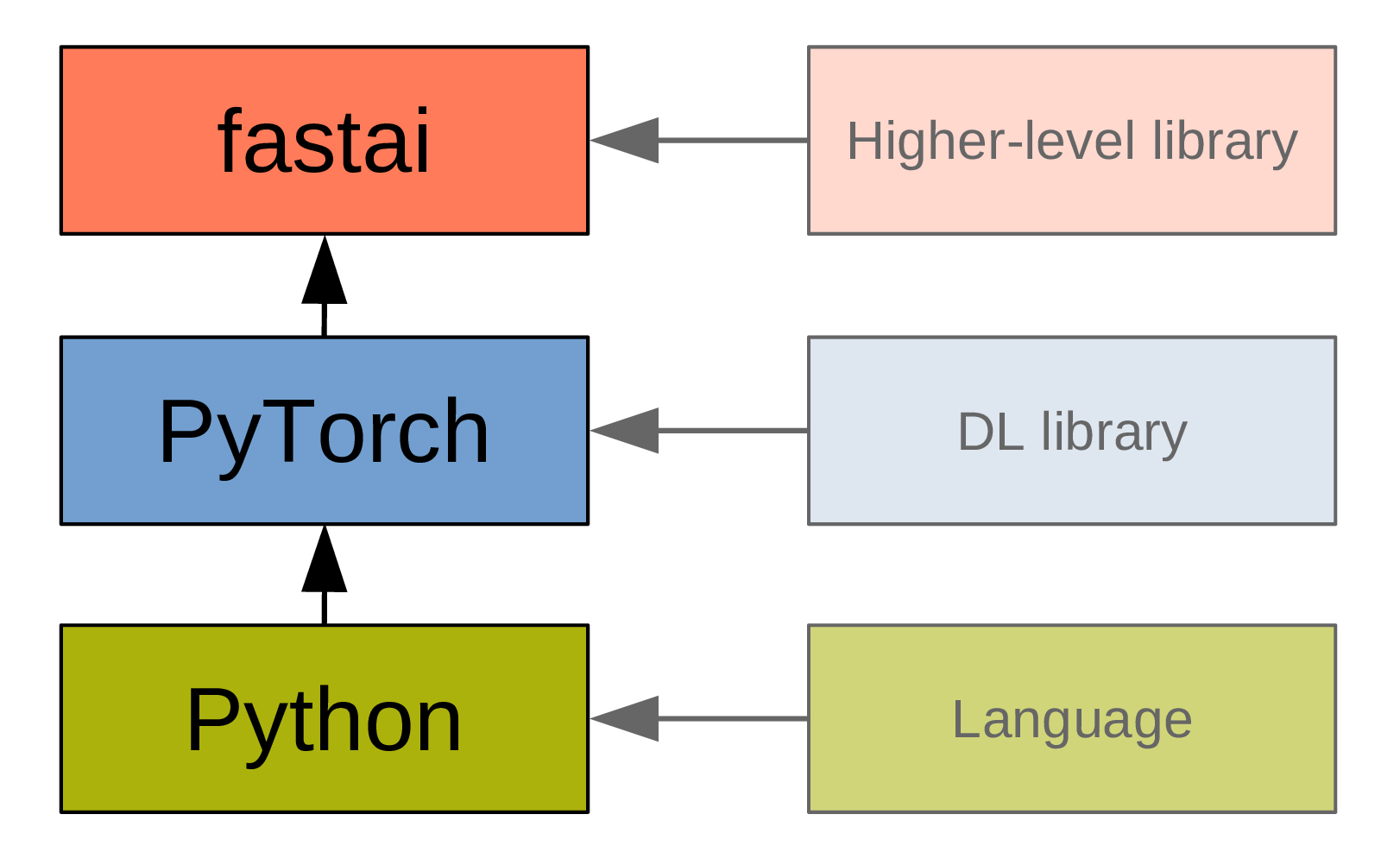
PyTorch

- Very Pythonic.
- Widely used in research.
fastai
fastai
is a deep learning library that builds on top of PyTorch, adding a higher level of functionality.
[It] is organized around two main design goals: to be approachable and rapidly productive, while also being deeply hackable and configurable.
Resources
Documentation
Manual
Tutorials
Peer-reviewed paper
Book
Paperback version
Free MOOC version of part 1 of the book
Jupyter notebooks version of the book
Getting help
Basic workflow
- DataLoaders
Create iterators with the training and validation data.
- Learner
Train the model.
- Predict or visualize
Get predictions from our model.
Example: identifying painters
Two main types of models
- Classification
- Regression
Two main types of models
- Classification
- Regression
Load domain specific library
In our case, we need the vision library:
from fastai.vision.all import *Other domains available:
from fastai.text.all import *
from fastai.tabular.all import *
from fastai.collab import *
Note that import * is not recommended in Python outside the context of fastai.
DataLoaders
A fastai class.
A simple wrapper around the PyTorch DataLoader class with added functionality (a DataLoader creates batches of data and sends them to the CPU or GPU as you iterate through it).
Creates an object of class DataLoaders which contains a validation DataLoader and a training DataLoader.
DataLoaders
Using search_images_bing, a convenience function to download images from the Bing API (free registration required).
key = os.environ.get('AZURE_SEARCH_KEY', '<your-private-key>')DataLoaders
Let’s download paintings from Monet:
monet = search_images_bing(key, 'monet')
ims = monet.attrgot('content_url')
path = Path('dataset')
fns = get_image_files(path)
fnsNote that this last output is of a fastai class L: a Python list with added functionality.
DataLoaders
We can do the same with Van Gogh:
vangogh = search_images_bing(key, 'vangogh')
ims = vangogh.attrgot('content_url')
path = Path('dataset')
fns = get_image_files(path)
fnsDataLoaders
Data block API:
paintings = DataBlock(
    blocks=(ImageBlock, CategoryBlock),
    get_items=get_image_files,
    splitter=RandomSplitter(valid_pct=0.2, seed=42),
    get_y=parent_label,
    item_tfms=Resize(128))
DataLoaders
- blocks: types of inputs and labels
- get_items: how to get the list of items
- splitter: how to split the data between a validation set and a training set
- get_y: how to label the data
- item_tfms: item transformation
- batch_tfms: transformation of the whole batch. Very fast as this happens in the GPU
DataLoaders
- blocks: types of inputs and labels
- get_items: how to get the list of items
- splitter: how to split the data between a validation set and a training set
- get_y: how to label the data
- item_tfms: item transformation
- batch_tfms: transformation of the whole batch. Very fast as this happens in the GPU
valid_pct=0.2: keep a validation set (20% of the data) to test the model.
Major pitfall: over-fitting

Major pitfall: over-fitting
- Training too long
- Training without enough data
- Too many parameters
DataLoaders
dls = paintings.dataloaders(path)We now have our DataLoaders object dls.
Let’s have a look at 4 items:
dls.valid.show_batch(max_n=4, nrows=1)
DataLoaders
To standardize the size of images, Resize cropped them, but there are alternative methods:
Squish
paintings = paintings.new(item_tfms=Resize(128, ResizeMethod.Squish))
dls = paintings.dataloaders(path)
dls.valid.show_batch(max_n=4, nrows=1)
DataLoaders
To standardize the size of images, Resize cropped them, but there are alternative methods:
Pad
paintings = paintings.new(item_tfms=Resize(128, ResizeMethod.Pad,
                                           pad_mode='zeros'))
dls = paintings.dataloaders(path)
dls.valid.show_batch(max_n=4, nrows=1)
Learner
learn = cnn_learner(dls, resnet18, metrics=error_rate)
learn.fine_tune(4)
Transfer learning
Repurposing pretrained models.
- Less data needed
- Less computing time needed
- Leads to better accuracy
Results
| epoch | train_loss | valid_loss | error_rate | time |
|---|---|---|---|---|
| 0 | 0.398155 | 0.167293 | 0.068152 | 00:03 |
| 1 | 0.204518 | 0.135118 | 0.050011 | 00:02 |
| 2 | 0.199835 | 0.099103 | 0.040012 | 00:05 |
| 3 | 0.179214 | 0.046119 | 0.025813 | 00:03 |
Getting into a lower level
Gradient descent
For each function, there is another function representing, not the values, but the rate of change of the values of the first function.
We need the gradients of the parameters with respect to the loss function to know in which direction and with which magnitude to adjust them at each step.
Automatic differentiation
To start tracking all operations performed on our model parameters:
params = tensor.requires_grad_()Gradient descent
Get the values predicted by our model with our parameters:
preds = model(params)Calculate the loss:
loss = loss_func(preds, targets)Backpropagation:
loss.backward()Gradient descent
Get the gradients:
params.gradUpdate the parameters:
params.data -= params.grad.data * lr.datastops the gradient from being calculated on this operation.lr: learning rate.
Usually between 0.0001 and 1.
Deeper networks are more bumpy and require lower learning rates (e.g. 0.01 instead of 0.1).
Gradient descent
Get the gradients:
params.gradUpdate the parameters:
params.data -= params.grad.data * lr.datastops the gradient from being calculated on this operation.lr: learning rate.
Reset the gradient:
params.grad = NoneGradient descent
Putting it all together:
def apply_step(params, prn=True):
    preds = model(params)
    loss = loss_func(preds, targets)
    loss.backward()
    params.data -= params.grad.data * lr
    params.grad = None
    if prn: print(loss.item())
    return preds

for i in range(4): apply_step(params)
Data bias
Bias is always present in data.
Document the limitations and scope of your data as best as possible.
Problems to watch for:
- Out of domain data: data used for training are not relevant to the model application.
- Domain shift: model becoming inadapted as conditions evolve.
- Feedback loop: initial bias exacerbated over the time.
The last one is particularly problematic whenever the model outputs the next round of data based on interactions of the current round of data with the real world.
Solution: ensure there are human circuit breakers and oversight.