AI, ML, DL:
Concepts

Machine learning
History
1943: W. McCulloch & W. Pitts—mathematical model of artificial neuron
1961: F. Rosenblatt—perceptron
1961: A. Samuel—checkers program
1986: J. McClelland, D. Rumelhart & PDP Research Group—book
Parallel Distributed Processing
Dominant approach:
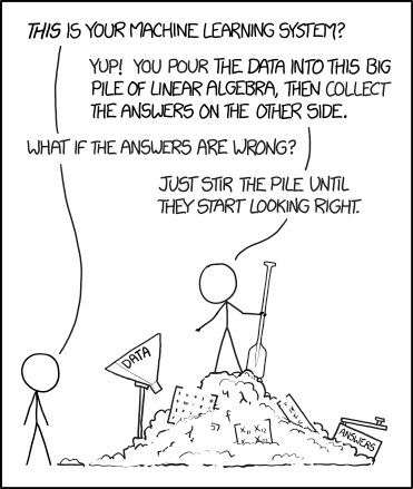
Dominant approach:
Example in image recognition:
Rather than coding explicitly all the possible ways—pixel by pixel—that a picture can represent an object, image/label pairs are fed to a neural network
Parameters get adjusted in an iterative and automated manner
Neurons
Schematic from <a href="https://commons.wikimedia.org/w/index.php?curid=1474927" target="_blank">Dhp1080, Wikipedia</a>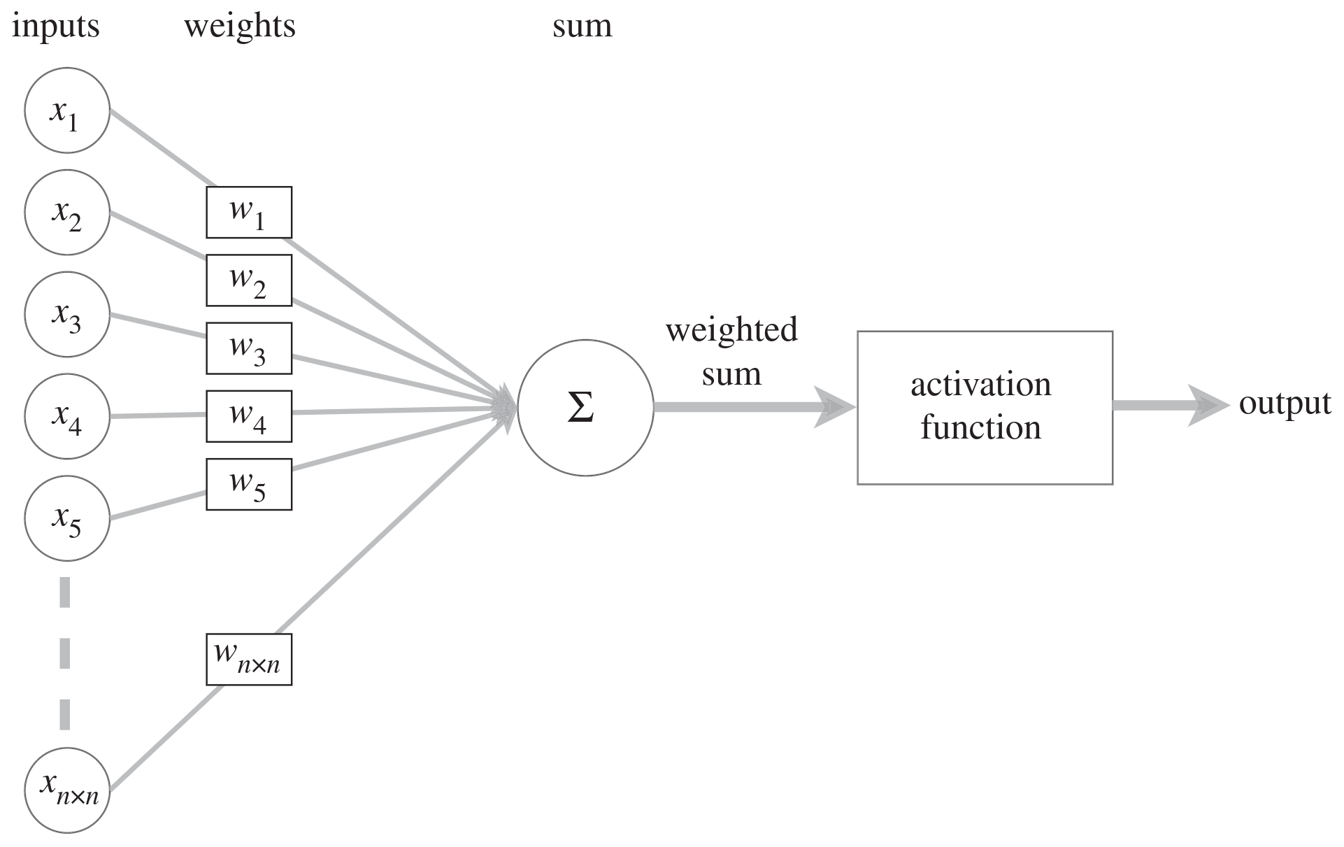
Modified from <a href="https://royalsocietypublishing.org/doi/10.1098/rsta.2019.0163" target="_blank">O.C. Akgun & J. Mei 2019</a>
Neurons
Schematic from <a href="https://commons.wikimedia.org/w/index.php?curid=1474927" target="_blank">Dhp1080, Wikipedia</a>
Modified from <a href="https://royalsocietypublishing.org/doi/10.1098/rsta.2019.0163" target="_blank">O.C. Akgun & J. Mei 2019</a>Biological neuron: an electrically excitable cell receives information through the dendrites & transmits a compiled output through the axons
Neurons
Schematic from <a href="https://commons.wikimedia.org/w/index.php?curid=1474927" target="_blank">Dhp1080, Wikipedia</a>
Modified from <a href="https://royalsocietypublishing.org/doi/10.1098/rsta.2019.0163" target="_blank">O.C. Akgun & J. Mei 2019</a>Artificial neuron: the weighted sum of a set of numeric inputs is passed through an activation function before yielding a numeric output
Activation
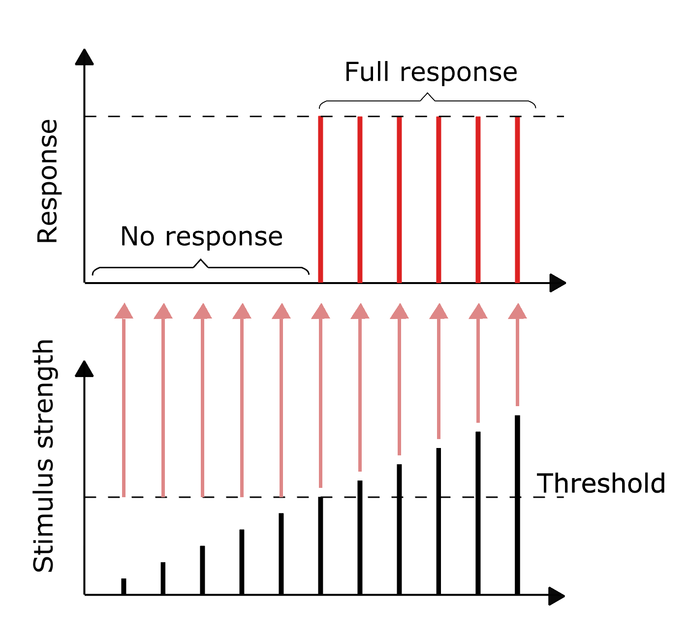
Modified from <a href="https://commons.wikimedia.org/w/index.php?curid=78013076">Blacktc, Wikimedia</a>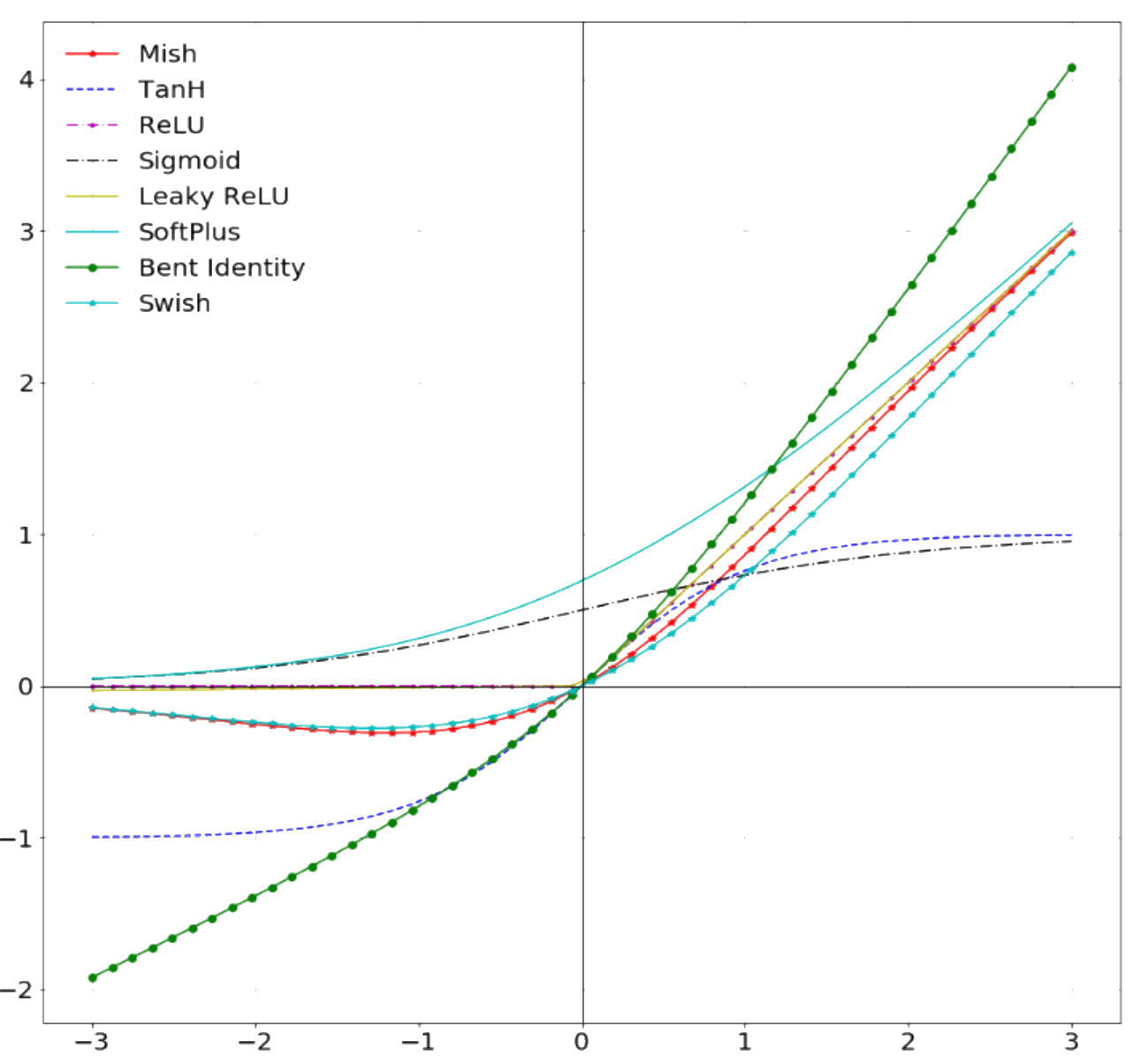
From <a href="https://arxiv.org/abs/1908.08681">Diganta Misra 2019</a>
Activation

Modified from <a href="https://commons.wikimedia.org/w/index.php?curid=78013076">Blacktc, Wikimedia</a>
From <a href="https://arxiv.org/abs/1908.08681">Diganta Misra 2019</a>Biological neuron: all-or-nothing action potential; greater stimuli don’t produce stronger signals but increase firing frequency
Activation

Modified from <a href="https://commons.wikimedia.org/w/index.php?curid=78013076">Blacktc, Wikimedia</a>
From <a href="https://arxiv.org/abs/1908.08681">Diganta Misra 2019</a>Artificial neuron: many activation functions have been tried; choices based on problem & available computing budget
Softmax activation function
\[\sigma(\mathbf{z})_i=\frac{e^{z_i}}{\sum_{j=1}^{K}e^{z_j}}\] \[\text{ for }i=1,…,K\text{ and }\mathbf{z}=(z_1,…,z_K)\in\mathbb{R}^K\]
(\(\mathbb{R}\) represents the set of real numbers)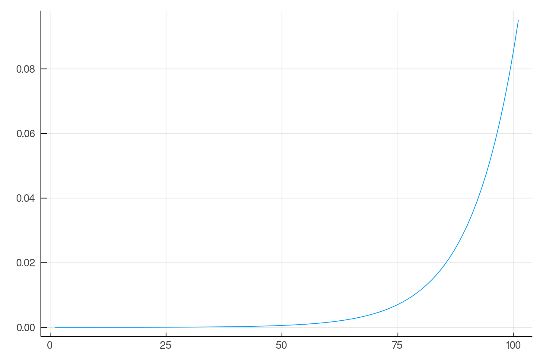
Vector of real numbers → vector of numbers between 0 and 1 which add to 1
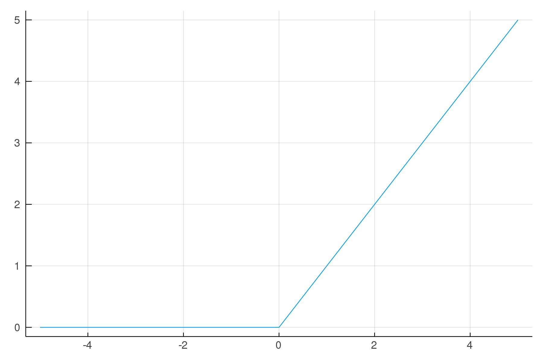
Relu: rectifier activation function
\[f(x) = max(0, x)\]
Neural networks

Image by <a href="https://news.berkeley.edu/2020/03/19/high-speed-microscope-captures-fleeting-brain-signals/" target="_blank">Na Ji, UC Berkeley</a>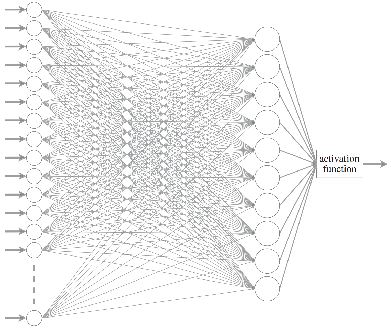
Modified from <a href="https://royalsocietypublishing.org/doi/10.1098/rsta.2019.0163" target="_blank">O.C. Akgun & J. Mei 2019</a>Neural networks

Image by <a href="https://news.berkeley.edu/2020/03/19/high-speed-microscope-captures-fleeting-brain-signals/" target="_blank">Na Ji, UC Berkeley</a>
Modified from <a href="https://royalsocietypublishing.org/doi/10.1098/rsta.2019.0163" target="_blank">O.C. Akgun & J. Mei 2019</a>Biological network: tremendously complex organization
Neural networks

Image by <a href="https://news.berkeley.edu/2020/03/19/high-speed-microscope-captures-fleeting-brain-signals/" target="_blank">Na Ji, UC Berkeley</a>
Modified from <a href="https://royalsocietypublishing.org/doi/10.1098/rsta.2019.0163" target="_blank">O.C. Akgun & J. Mei 2019</a>Natural network: organized in layers
Neural networks
Single layer of artificial neurons → Unable to learn even some of the simple mathematical functions (Marvin Minsky & Seymour Papert)
Two layers → Theoretically can approximate any math model, but in practice very slow
More layers → Deeper networks
deep learning = two or more layers
How do neural networks learn?
Building a model

First, we need an architecture: size, depth, types of layers, etc.
This is set before training and does not change.
Building a model

Then we need parameters.
Those are set to some initial values, but will change during training.
Training a model
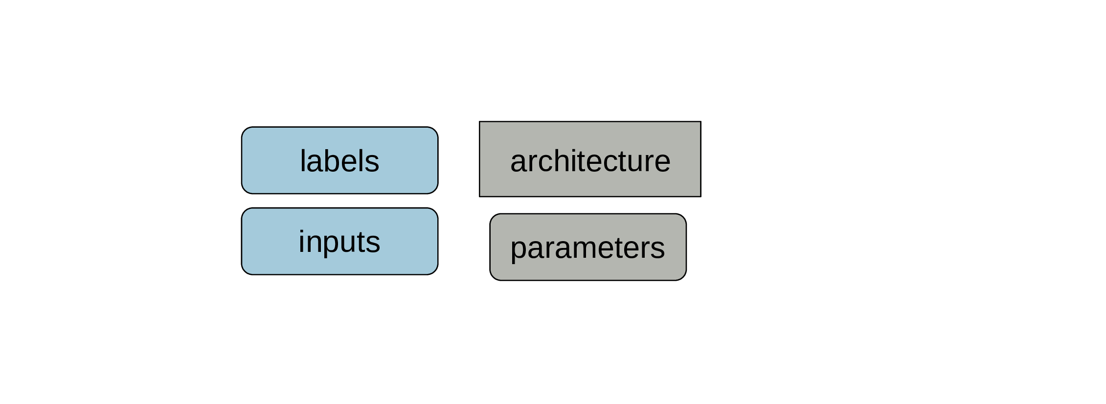
To train the model, we need labelled examples (input/output pairs).
Training a model

The inputs are features: characteristics describing our data.
The outputs are labels: the variable we are predicting, also called targets.
Training a model
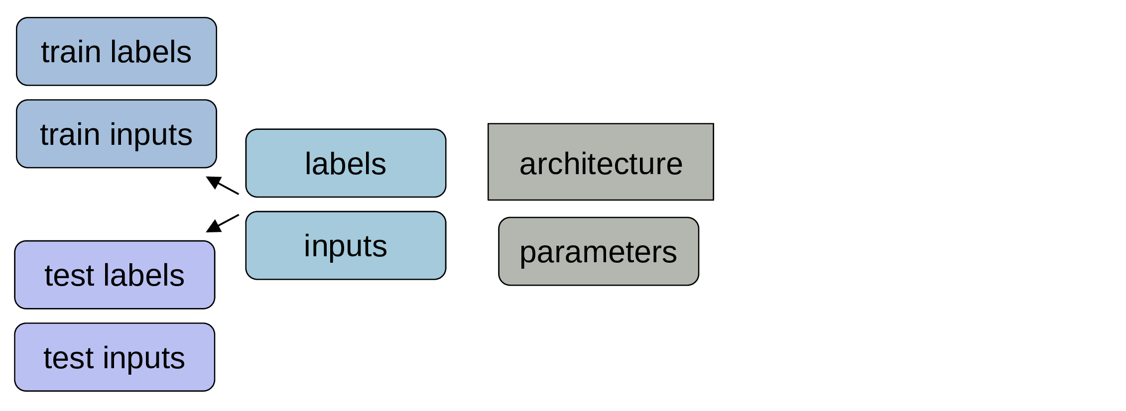
We split the labelled data into a training set (often c. 80%) & a testing set (the rest).
Training a model
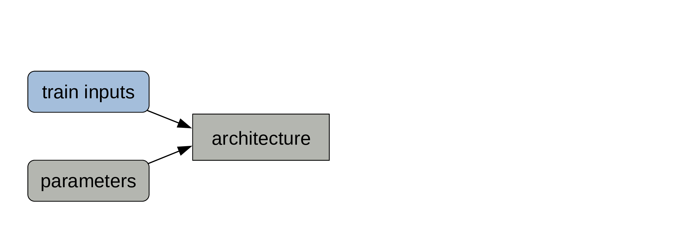
Training inputs and parameters are fed to the architecture.
Training a model
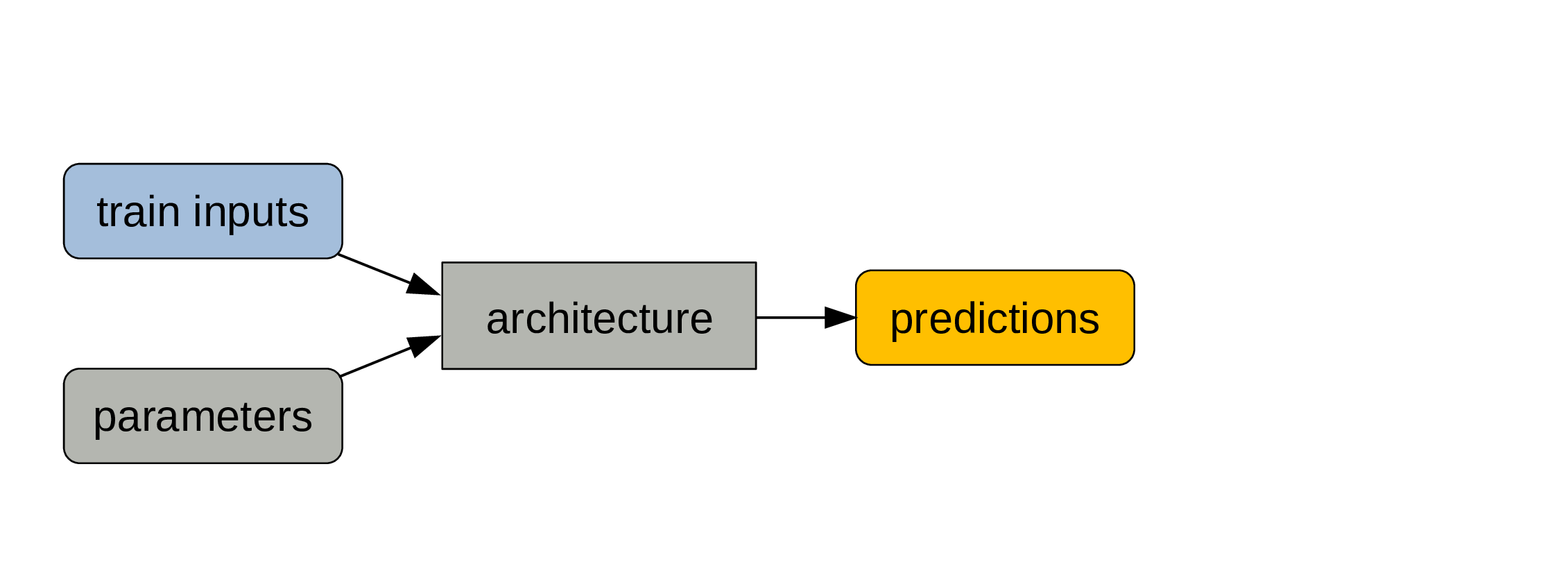
We get predictions as outputs.
Training a model
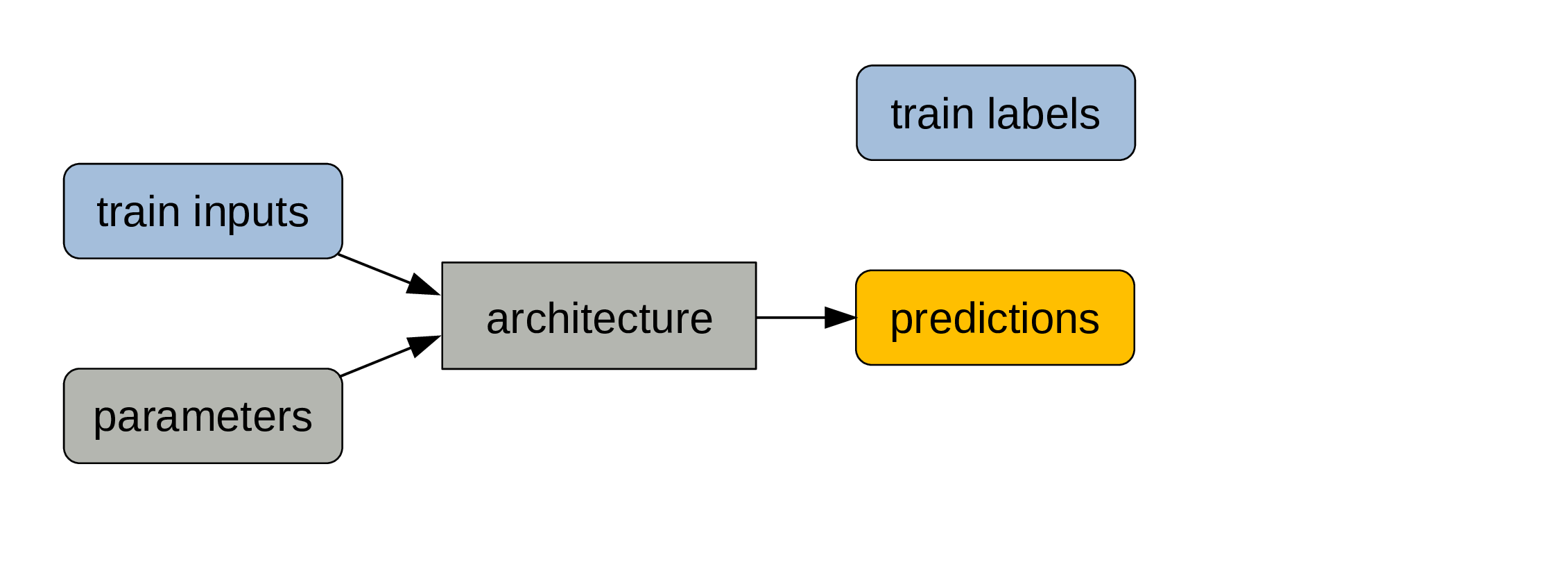
A metric (e.g. error rate) compares predictions & training labels: this is a measure of model performance.
Training a model
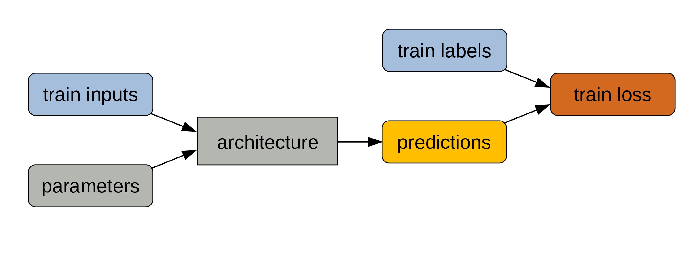
Because it is not always sensitive enough to changes in parameter values,
we compute a loss function …
Training a model
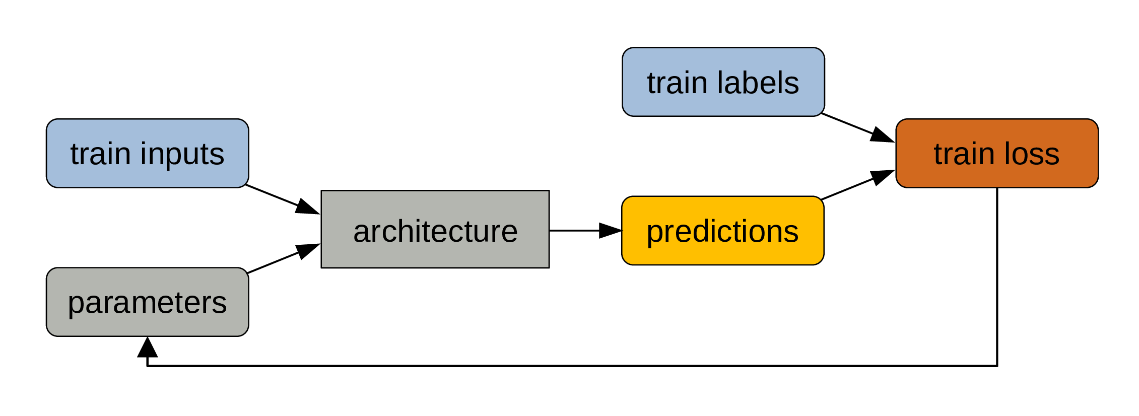
… which allows to adjust the parameters slightly through backpropagation.
This cycle gets repeated at each step.
Training a model
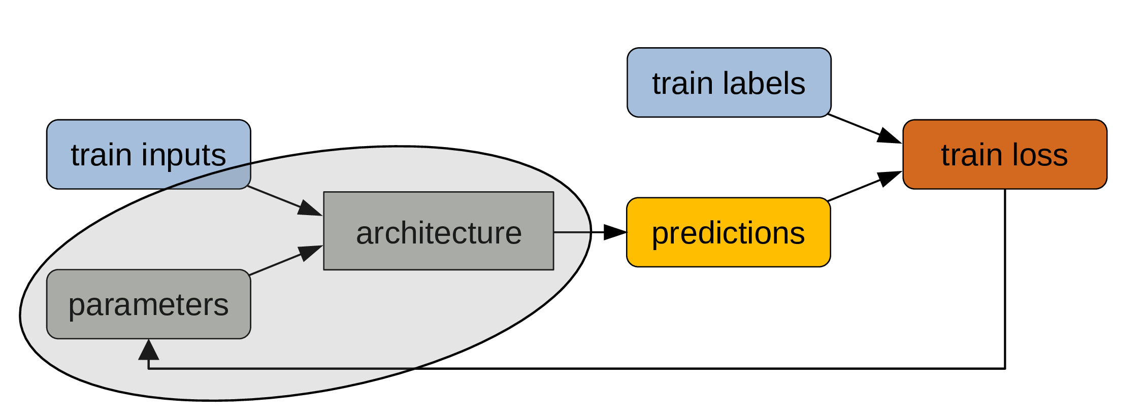
At the end of the training process, what matters is the combination of architecture and trained parameters.
A model
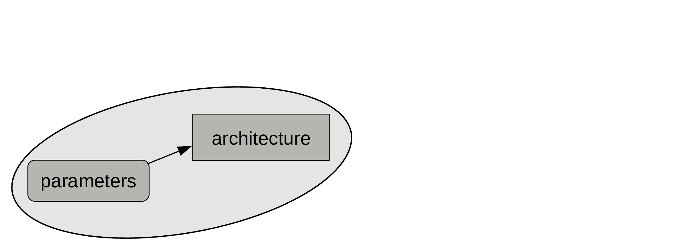
That’s what constitute a model.
A model
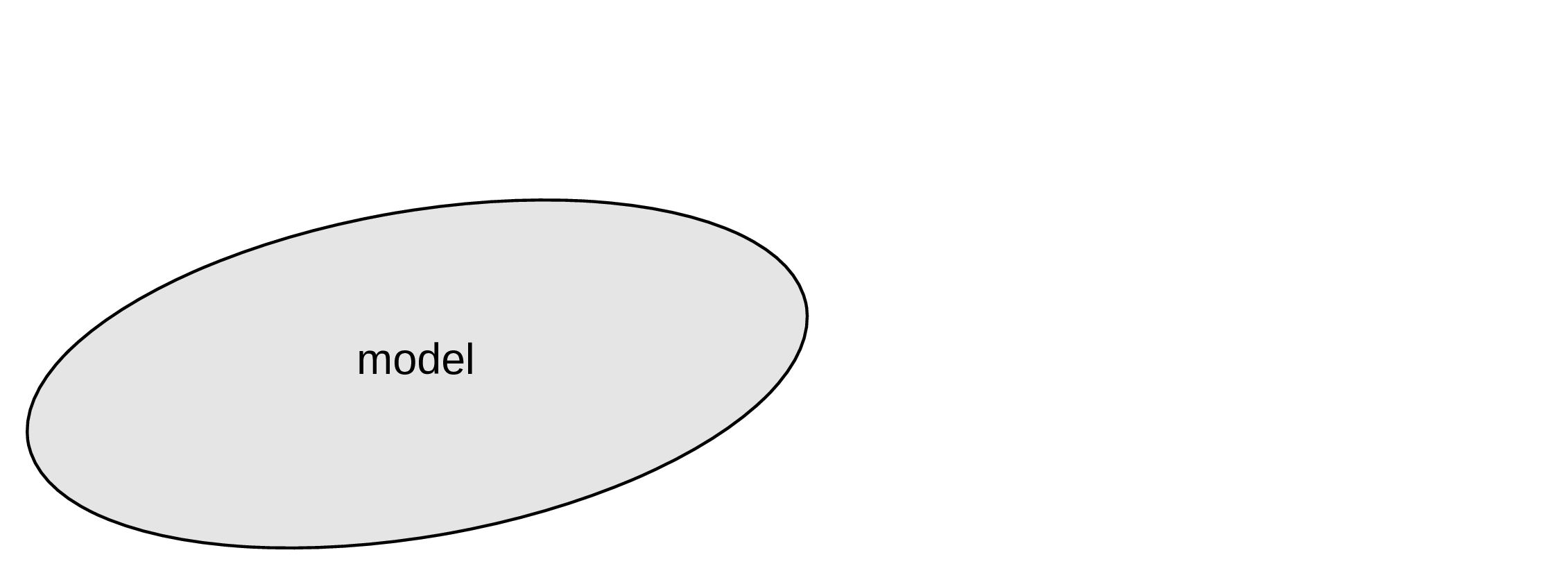
A model can be considered as a regular program.
Testing a model
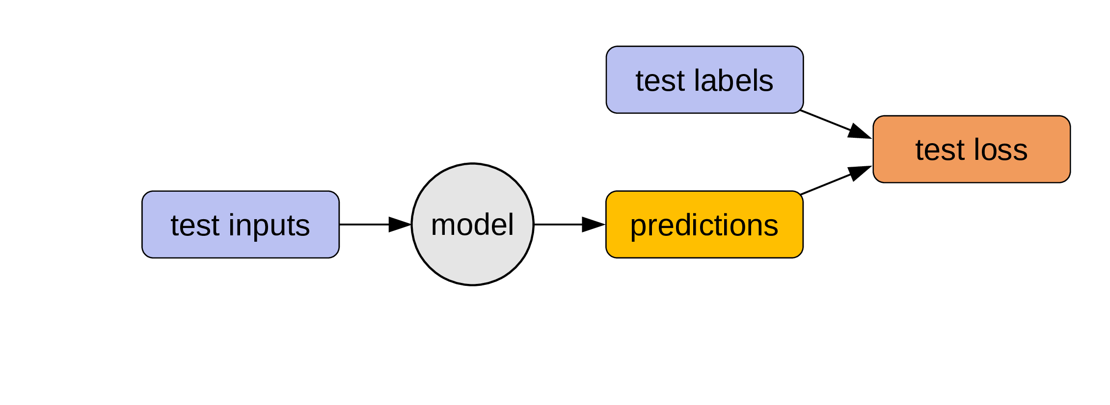
We test the model on labelled data it has never seen: the testing data.
No training data is used here!
Testing a model

The testing loss informs us on how well our model performs with data it was not trained on.
Using a model
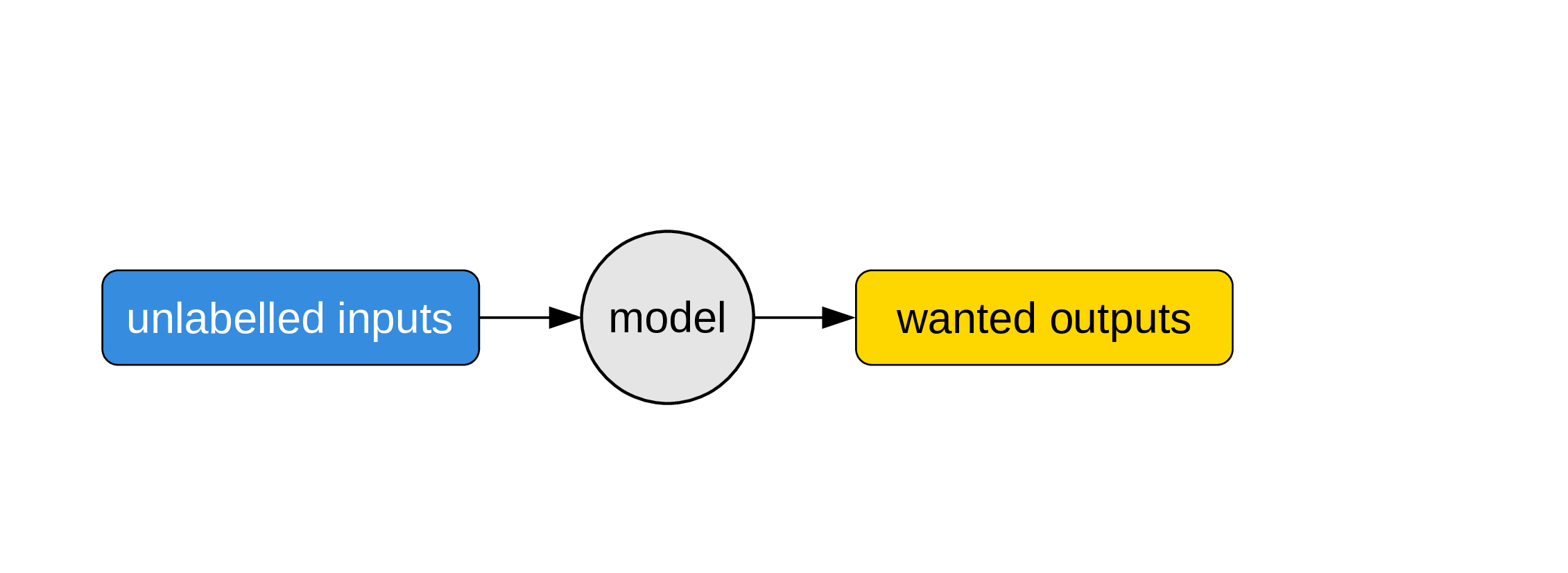
Finally, the model can be used to obtain outputs we really care about from unlabelled inputs. We are now using it just like a regular program.