Our first neural network
with PyTorch

WestGrid Summer School

Marie-Hélène Burle

PyTorch’s packages

PyTorch comes with several packages that make working with neural nets easy.

In the previous lesson, we learnt about torch.autograd which allows automatic calculation of gradients during backpropagation.

This lesson introduces torch.nn and torch.optim. They are often imported with:

import torch.nn as nn
import torch.optim as optim

torch.nn.functional

The torch.nn.functional module contains all the functions of the torch.nn package. By convention, it is imported as F:

import torch.nn.functional as F

These functions include loss functions, activation functions, pooling functions … i.e. all the functions that are used in the building and training of a neural net. Since torch.autograd can be used on any callable object, you can also create and use your own functions.

Loss functions

In our previous lesson, we calculated a loss function manually with:

loss = (predicted - real).pow(2).sum()

Loss functions

Within torch.nn.functional, you can select from a large range of loss functions:

binary_cross_entropy to calculate the binary cross entropy between the target and the output
binary_cross_entropy_with_logits to calculate the binary cross entropy between target and output logits
poisson_nll_loss for Poisson negative log likelihood loss
…

Go to the documentation for a full list.

Loss functions

Example:

If we want to use the negative log likelihood loss function, we can run:

loss = F.nll_loss(predicted, real)

Activation functions

As mentioned earlier, torch.nn.functional also has activation functions.

Examples:

ReLU can be called with torch.nn.functional.relu()
Softmax with torch.nn.functional.softmax()

torch.nn.Module

torch.nn.Module is the base class for all neural network modules. To build your model, you create a subclass of torch.nn.Module:

class Net(nn.Module):
	def __init__(self):
		super(Net, self).__init__()

Python’s class inheritance gives our subclass all the functionality of torch.nn.Module while allowing us to customize it.

torch.nn.Module

Then, you can create submodules and assign them as attributes:

class Net(nn.Module):
	def __init__(self):
		super(Net, self).__init__()
		self.fc1 = nn.Linear(784, 128)
		self.fc2 = nn.Linear(128, 10)

If this Python syntax is obscure to you, you should have a look at the answers to this question , as well as this answer to a similar question .

torch.nn.Module

Finally, you define the method for the forward pass in your subclass of torch.nn.Module:

class Net(nn.Module):
	def __init__(self):
		super(Net, self).__init__()
		self.fc1 = nn.Linear(784, 128)
		self.fc2 = nn.Linear(128, 10)

	def forward(self, x):
		x = torch.flatten(x, 1)
		x = self.fc1(x)
		x = F.relu(x)
		x = self.fc2(x)
		output = F.log_softmax(x, dim=1)
		return output

torch.nn.Module

Now, we have our network architecture, so we can create an instance of it:

model = Net()

Even better, we can send it to our device of choice (CPU or GPU):

model = Net().to(device)

torch.optim

The package torch.optim contains classic optimization algorithms such as optim.SGD(), optim.Adam(), or optim.Adadelta().

To use them, you define an optimizer with one such algorithms:

optimizer = optim.Adadelta(model.parameters(), lr=1.0)

Then use:

optimizer.zero_grad()  # resets the gradient to 0
optimizer.step()

Let’s try to build a NN
to classify the MNIST

Our script

ssh into the training cluster:

ssh userxxx@uu.c3.ca

Create a directory for this project and cd into it:

mkdir mnist; cd mnist

Start a first Python script:

nano mlp.py   # use the text editor of your choice

Let’s start with an MLP

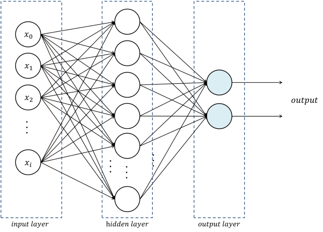
Let’s start with the simplest possible neural net: a multilayer perceptron (MLP) .

It is a feed-forward (i.e. no loop), fully-connected (i.e. each neuron of one layer is connected to all the neurons of the adjacent layers) neural network with a single hidden layer.

Load all the modules we need

import torch
import torch.nn as nn
import torch.nn.functional as F
import torch.optim as optim
from torchvision import datasets, transforms
from torch.optim.lr_scheduler import StepLR

Our model

class Net(nn.Module):
	def __init__(self):
		super(Net, self).__init__()
		self.fc1 = nn.Linear(784, 128)
		self.fc2 = nn.Linear(128, 10)

	def forward(self, x):
		x = torch.flatten(x, 1)
		x = self.fc1(x)
		x = F.relu(x)
		x = self.fc2(x)
		output = F.log_softmax(x, dim=1)
		return output

Our training function

def train(model, device, train_loader, optimizer, epoch):
    model.train()
    for batch_idx, (data, target) in enumerate(train_loader):
        data, target = data.to(device), target.to(device)
        optimizer.zero_grad()
        output = model(data)
        loss = F.nll_loss(output, target)
        loss.backward()
        optimizer.step()
        if batch_idx % 10 == 0:
            print('Train Epoch: {} [{}/{} ({:.0f}%)]\tLoss: {:.6f}'.format(
                epoch, batch_idx * len(data), len(train_loader.dataset),
                100. * batch_idx / len(train_loader), loss.item()))

Our testing function

def test(model, device, test_loader):
    model.eval()
    test_loss = 0
    correct = 0
    with torch.no_grad():
        for data, target in test_loader:
            data, target = data.to(device), target.to(device)
            output = model(data)
            test_loss += F.nll_loss(output, target, reduction='sum').item()  # sum up batch loss
            pred = output.argmax(dim=1, keepdim=True)  # get the index of the max log-probability
            correct += pred.eq(target.view_as(pred)).sum().item()

    test_loss /= len(test_loader.dataset)

    print('\nTest set: Average loss: {:.4f}, Accuracy: {}/{} ({:.0f}%)\n'.format(
        test_loss, correct, len(test_loader.dataset),
        100. * correct / len(test_loader.dataset)))

Our training settings

def main():
    epochs = 3
    torch.manual_seed(1)
    device = torch.device('cpu')

    transform = transforms.Compose([
        transforms.ToTensor(),
        transforms.Normalize((0.1307,), (0.3081,))
    ])

    train_data = datasets.MNIST(
        '~/projects/def-sponsor00/data',
        train=True, download=True, transform=transform)

    test_data = datasets.MNIST(
        '~/projects/def-sponsor00/data',
        train=False, transform=transform)

    train_loader = torch.utils.data.DataLoader(train_data, batch_size=64)
    test_loader = torch.utils.data.DataLoader(test_data, batch_size=1000)
    model = Net().to(device)
    optimizer = optim.Adadelta(model.parameters(), lr=1.0)
    scheduler = StepLR(optimizer, step_size=1, gamma=0.7)

    for epoch in range(1, epochs + 1):
        train(model, device, train_loader, optimizer, epoch)
        test(model, device, test_loader)
        scheduler.step()

Our training settings

We will only run our model over 3 epochs to save time. Obviously, you normally would run it much longer.

We are using CPUs.

We will use the Adadelta algorithm as optimizer.

Running the model

Finally, we run the whole model by running main():

main()

Let’s try our script

Now is the time to submit our script to Slurm to test it!

Slurm script

Write an mlp.sh script:

#!/bin/bash
#SBATCH --time=0:5:0
#SBATCH --cpus-per-task=1
#SBATCH --mem=3G
#SBATCH --output=%x_%j.out
#SBATCH --error=%x_%j.err

# Activate your virtual env
source ~/env/bin/activate

# Run your Python script
python ~/mnist/mlp.py

Submit the job to Slurm

sbatch mlp.sh

Monitor its status with:

sq

On to a CNN

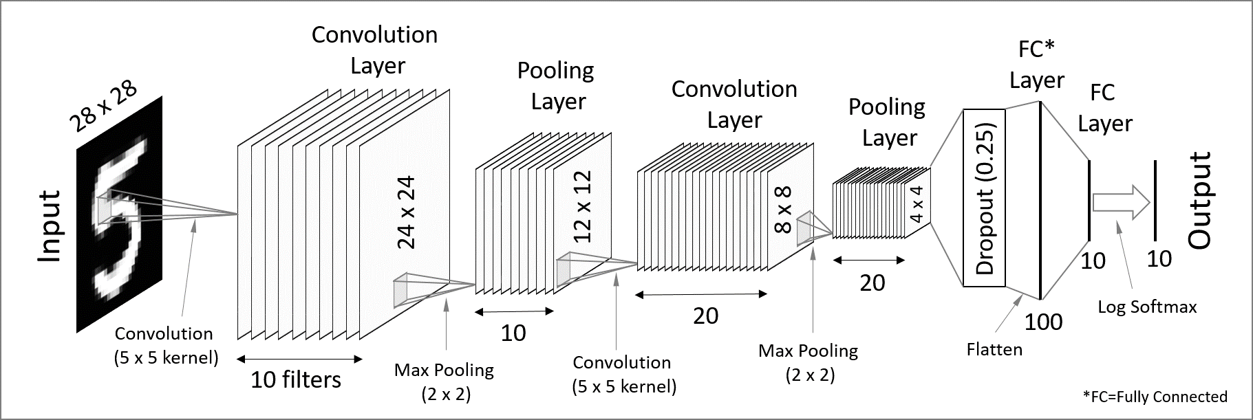
Let’s step this up and build a CNN. Convolutional Neural Networks are particularly well-suited to image data.

The figure below is not an exact scheme of the model we will build, but it represents a similar model made of convolution, pooling, and fully-connected layers.

*From Programming Journeys by Rensu Theart*

CNN script

Our new script will be very similar to mlp.py: we will only change the model architecture. So you can copy mlp.py and edit the copy:

cp mlp.py cnn.py
nano cnn.py

Our new model architecture

class Net(nn.Module):
	def __init__(self):
		super(Net, self).__init__()
		self.conv1 = nn.Conv2d(1, 32, 3, 1)
		self.conv2 = nn.Conv2d(32, 64, 3, 1)
		self.dropout1 = nn.Dropout2d(0.25)
		self.dropout2 = nn.Dropout2d(0.5)
		self.fc1 = nn.Linear(9216, 128)
		self.fc2 = nn.Linear(128, 10)

	def forward(self, x):
		x = self.conv1(x)
		x = F.relu(x)
		x = self.conv2(x)
		x = F.relu(x)
		x = F.max_pool2d(x, 2)
		x = self.dropout1(x)
		x = torch.flatten(x, 1)
		x = self.fc1(x)
		x = F.relu(x)
		x = self.dropout2(x)
		x = self.fc2(x)
		output = F.log_softmax(x, dim=1)
		return output

Slurm script

Write a cnn.sh script. We need more time here as a CNN will take longer to run.

#!/bin/bash
#SBATCH --time=0:15:0
#SBATCH --cpus-per-task=1
#SBATCH --mem=3G
#SBATCH --output=%x_%j.out
#SBATCH --error=%x_%j.err

# Activate your virtual env
source ~/env/bin/activate

# Run your Python script
python ~/mnist/cnn.py

Submit the job to Slurm

sbatch cnn.sh

Monitor its status with:

sq

Our first neural network with PyTorch

WestGrid Summer School

Marie-Hélène Burle

PyTorch’s packages

torch.nn.functional

Loss functions

Loss functions

Loss functions

Activation functions

torch.nn.Module

torch.nn.Module

torch.nn.Module

torch.nn.Module

torch.optim

Let’s try to build a NN to classify the MNIST

Our script

Let’s start with an MLP

Load all the modules we need

Our model

Our training function

Our testing function

Our training settings

Our training settings

Running the model

Let’s try our script

Slurm script

Submit the job to Slurm

On to a CNN

CNN script

Our new model architecture

Slurm script

Submit the job to Slurm

Questions?

Our first neural network
with PyTorch

Let’s try to build a NN
to classify the MNIST