Everything you wanted to know (and more) about
PyTorch tensors
Marie-Hélène Burle
Marie-Hélène Burle
training@westgrid.ca
January 19, 2022

Using tensors locally
You need to have Python & PyTorch installed Additionally, you might want to use an IDE such as elpy if you are an Emacs user, JupyterLab , etc.
For the time being, you might have to use it with Python 3.9
Using tensors on CC clusters
In the cluster terminal:
avail_wheels "torch*" # List available wheels & compatible Python versions
module avail python	  # List available Python versions
module load python/3.9.6             # Load a sensible Python version
virtualenv --no-download env         # Create a virtual env
source env/bin/activate		         # Activate the virtual env
pip install --no-index --upgrade pip # Update pip
pip install --no-index torch		 # Install PyTorch
You can then launch jobs with sbatch or salloc
Leave the virtual env with the command: deactivate
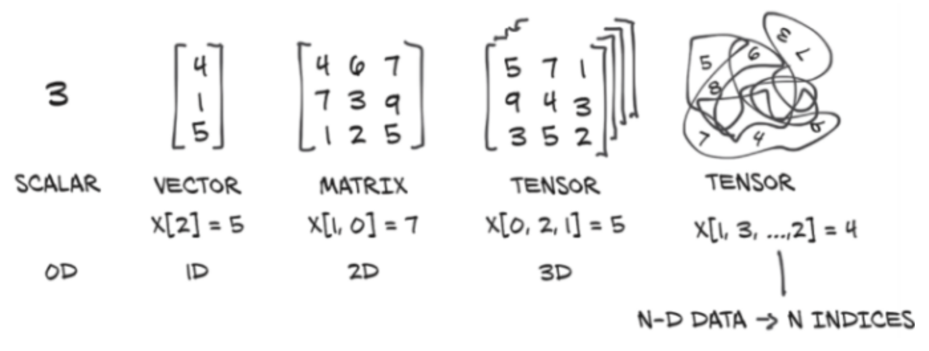
- What is a PyTorch tensor?
- Memory storage
- Data type (dtype)
- Basic operations
- Working with NumPy
- Linear algebra
- Harvesting the power of GPUs
- Distributed operations
- What is a PyTorch tensor?
- Memory storage
- Data type (dtype)
- Basic operations
- Working with NumPy
- Linear algebra
- Harvesting the power of GPUs
- Distributed operations
ANN do not process information directly
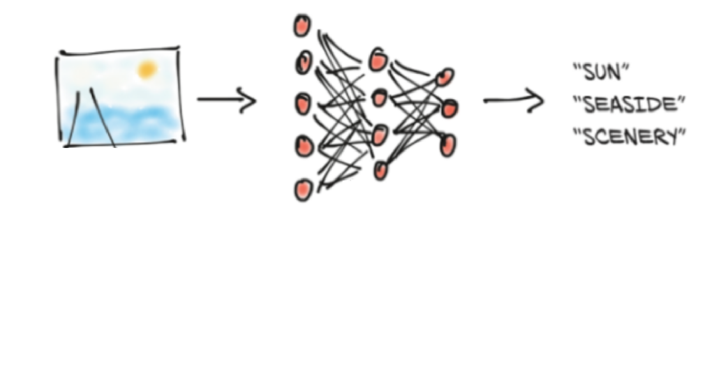
It needs to be converted to numbers
All these numbers need to be stored
in a data structure
in a data structure
Why a new object when NumPy ndarray already exists?
Can run on accelerators (GPUs, TPUs…)
Keep track of computation graphs, allowing automatic differentiation
Future plan for sharded tensors to run distributed computations
What is a PyTorch tensor?
PyTorch is foremost a deep learning library
In deep learning, the information contained in objects of interest (e.g. images, texts, sounds) is converted to floating-point numbers (e.g. pixel values, token values, frequencies)
As this information is complex, multiple dimensions are required (e.g. two dimensions for the width & height of an image, plus one dimension for the RGB colour channels)
Additionally, items are grouped into batches to be processed together, adding yet another dimension
Multidimensional arrays are thus particularly well suited for deep learningWhat is a PyTorch tensor?
Artificial neurons perform basic computations on these tensors
Their number however is huge & computing efficiency is paramount
GPUs/TPUs are particularly well suited to perform many simple operations in parallel
The very popular NumPy library has, at its core, a mature multidimensional array object well integrated into the scientific Python ecosystem
But the PyTorch tensor has additional efficiency characteristics ideal for machine learning & it can be converted to/from NumPy’s ndarray if needed
- What is a PyTorch tensor?
- Memory storage
- Data type (dtype)
- Basic operations
- Working with NumPy
- Linear algebra
- Harvesting the power of GPUs
- Distributed operations
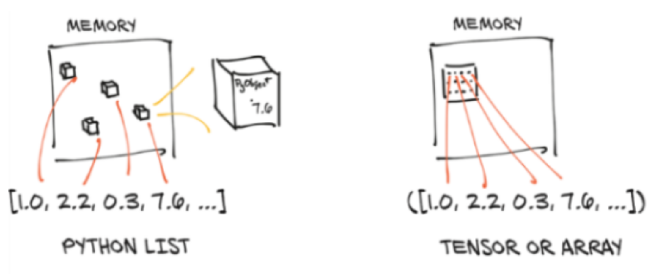
Efficient memory storage
In Python, collections (lists, tuples) are groupings of boxed Python objects
PyTorch tensors & NumPy ndarrays are made of unboxed C numeric types
Efficient memory storage
They are usually contiguous memory blocks, but the main difference is that they are unboxed: floats will thus take 4 (32-bit) or 8 (64-bit) bytes each
Boxed values take up more memory
(memory for the pointer + memory for the primitive)
Implementation
Under the hood, the values of a PyTorch tensor are stored as a torch.Storage instance which is a one-dimensional array
import torch
t = torch.arange(10.).view(2, 5); print(t) # Functions explained latertensor([[ 0., 1., 2., 3., 4.],
[ 5., 6., 7., 8., 9.]])Implementation
storage = t.storage(); print(storage) 0.0
1.0
2.0
3.0
4.0
5.0
6.0
7.0
8.0
9.0
[torch.FloatStorage of size 10]Implementation
The storage can be indexed
storage[3]3.0Implementation
storage[3] = 10.0; print(storage) 0.0
1.0
2.0
10.0
4.0
5.0
6.0
7.0
8.0
9.0
[torch.FloatStorage of size 10]Implementation
To view a multidimensional array from storage, we need metadata :
- the size (shape in NumPy) sets the number of elements in each dimension
- the offset indicates where the first element of the tensor is in the storage
- the stride establishes the increment between each element
Storage metadata
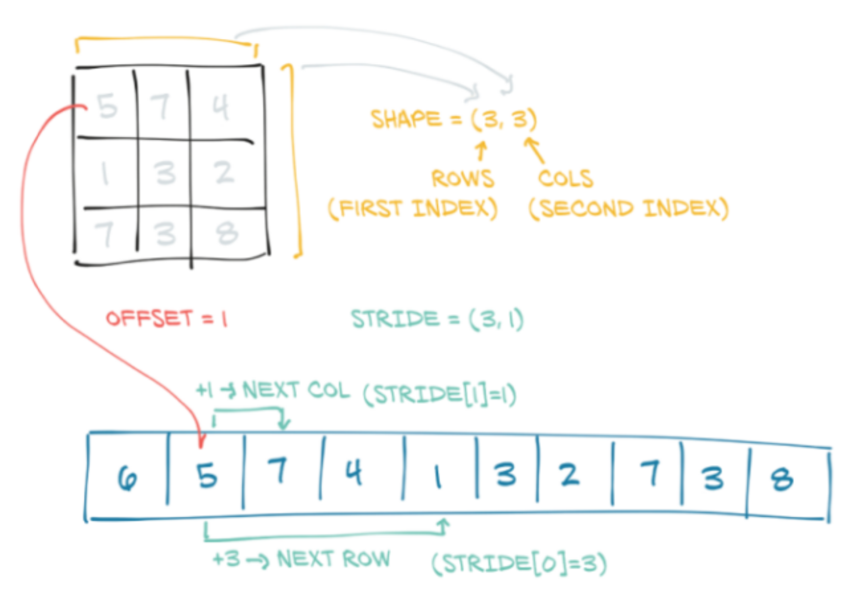
Storage metadata
t.size()
t.storage_offset()
t.stride()torch.Size([2, 5])
0
(5, 1)offset: 0
stride: (5, 1)
Storage metadata
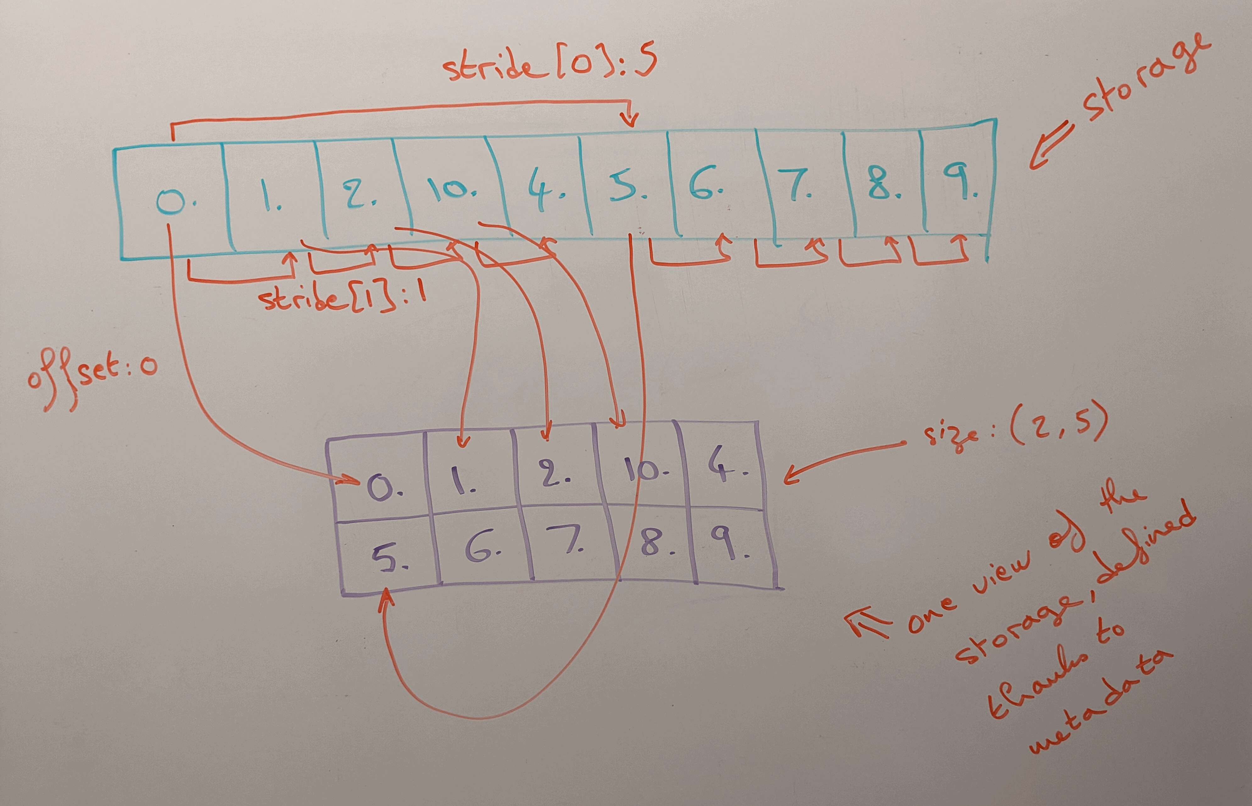
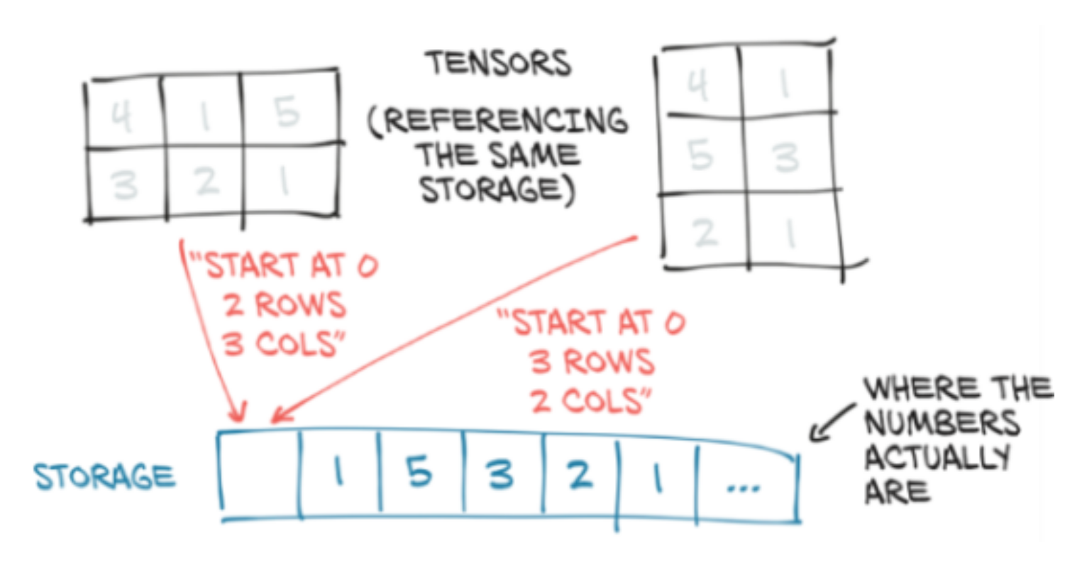
Sharing storage
Multiple tensors can use the same storage, saving a lot of memory since the metadata is a lot lighter than a whole new array
Transposing in 2 dimensions
t = torch.tensor([[3, 1, 2], [4, 1, 7]]); print(t)
t.size()
t.t()
t.t().size()tensor([[3, 1, 2],
[4, 1, 7]])
torch.Size([2, 3])
tensor([[3, 4],
[1, 1],
[2, 7]])
torch.Size([3, 2])Transposing in 2 dimensions
Transposing in higher dimensions
torch.t() is a shorthand for torch.transpose(0, 1):
torch.equal(t.t(), t.transpose(0, 1))TrueWhile torch.t() only works for 2D tensors, torch.transpose() can be used to transpose 2 dimensions in tensors of any number of dimensions
Transposing in higher dimensions
t = torch.zeros(1, 2, 3); print(t)

t.size()
t.stride()tensor([[[0., 0., 0.],
[0., 0., 0.]]])
torch.Size([1, 2, 3])
(6, 3, 1)Transposing in higher dimensions
t.transpose(0, 1)

t.transpose(0, 1).size()
t.transpose(0, 1).stride()tensor([[[0., 0., 0.]],
[[0., 0., 0.]]])
torch.Size([2, 1, 3])
(3, 6, 1) # Notice how transposing flipped 2 elements of the strideTransposing in higher dimensions
t.transpose(0, 2)

t.transpose(0, 2).size()
t.transpose(0, 2).stride()tensor([[[0.],
[0.]],
[[0.],
[0.]],
[[0.],
[0.]]])
torch.Size([3, 2, 1])
(1, 3, 6)Transposing in higher dimensions
t.transpose(1, 2)

t.transpose(1, 2).size()
t.transpose(1, 2).stride()tensor([[[0., 0.],
[0., 0.],
[0., 0.]]])
torch.Size([1, 3, 2])
(6, 1, 3)- What is a PyTorch tensor?
- Memory storage
- Data type (dtype)
- Basic operations
- Working with NumPy
- Linear algebra
- Harvesting the power of GPUs
- Distributed operations
Default dtype
Since PyTorch tensors were built with utmost efficiency in mind for neural networks, the default data type is 32-bit floating points
This is sufficient for accuracy & much faster than 64-bit floating points
List of PyTorch tensor dtypes
| torch.float16 / torch.half | 16-bit / half-precision floating-point | |
| torch.float32 / torch.float | 32-bit / single-precision floating-point | |
| torch.float64 / torch.double | 64-bit / double-precision floating-point | |
| torch.uint8 | unsigned 8-bit integers | |
| torch.int8 | signed 8-bit integers | |
| torch.int16 / torch.short | signed 16-bit integers | |
| torch.int32 / torch.int | signed 32-bit integers | |
| torch.int64 / torch.long | signed 64-bit integers | |
| torch.bool | boolean |
Checking & changing dtype
t = torch.rand(2, 3); print(t)
t.dtype   # Remember that the default dtype for PyTorch tensors is float32
t2 = t.type(torch.float64); print(t2) # If dtype ≠ default, it is printed
t2.dtypetensor([[0.8130, 0.3757, 0.7682],
[0.3482, 0.0516, 0.3772]])
torch.float32
tensor([[0.8130, 0.3757, 0.7682],
[0.3482, 0.0516, 0.3772]], dtype=torch.float64)
torch.float64- What is a PyTorch tensor?
- Memory storage
- Data type (dtype)
- Basic operations
- Working with NumPy
- Linear algebra
- Harvesting the power of GPUs
- Distributed operations
Creating tensors
torch.tensor: Input individual valuestorch.arange: Similar torangebut creates a 1D tensortorch.linspace: 1D linear scale tensortorch.logspace: 1D log scale tensortorch.rand: Random numbers from a uniform distribution on[0, 1)torch.randn: Numbers from the standard normal distributiontorch.randperm: Random permutation of integerstorch.empty: Uninitialized tensortorch.zeros: Tensor filled with0torch.ones: Tensor filled with1torch.eye: Identity matrix
Creating tensors
torch.manual_seed(0)  # If you want to reproduce the result
torch.rand(1)

torch.manual_seed(0)  # Run before each operation to get the same result
torch.rand(1).item() # Extract the value from a tensortensor([0.4963])
0.49625658988952637Creating tensors
torch.rand(1)
torch.rand(1, 1)
torch.rand(1, 1, 1)
torch.rand(1, 1, 1, 1)tensor([0.6984])
tensor([[0.5675]])
tensor([[[0.8352]]])
tensor([[[[0.2056]]]])Creating tensors
torch.rand(2)
torch.rand(2, 2, 2, 2)tensor([0.5932, 0.1123])
tensor([[[[0.1147, 0.3168],
[0.6965, 0.9143]],
[[0.9351, 0.9412],
[0.5995, 0.0652]]],
[[[0.5460, 0.1872],
[0.0340, 0.9442]],
[[0.8802, 0.0012],
[0.5936, 0.4158]]]])Creating tensors
torch.rand(2)
torch.rand(3)
torch.rand(1, 1)
torch.rand(1, 1, 1)
torch.rand(2, 6)tensor([0.7682, 0.0885])
tensor([0.1320, 0.3074, 0.6341])
tensor([[0.4901]])
tensor([[[0.8964]]])
tensor([[0.4556, 0.6323, 0.3489, 0.4017, 0.0223, 0.1689],
[0.2939, 0.5185, 0.6977, 0.8000, 0.1610, 0.2823]])Creating tensors
torch.rand(2, 4, dtype=torch.float64)  # You can set dtype
torch.ones(2, 1, 4, 5)tensor([[0.6650, 0.7849, 0.2104, 0.6767],
[0.1097, 0.5238, 0.2260, 0.5582]], dtype=torch.float64)
tensor([[[[1., 1., 1., 1., 1.],
[1., 1., 1., 1., 1.],
[1., 1., 1., 1., 1.],
[1., 1., 1., 1., 1.]]],
[[[1., 1., 1., 1., 1.],
[1., 1., 1., 1., 1.],
[1., 1., 1., 1., 1.],
[1., 1., 1., 1., 1.]]]])Creating tensors
t = torch.rand(2, 3); print(t)
torch.zeros_like(t)             # Matches the size of t
torch.ones_like(t)
torch.randn_like(t)tensor([[0.4051, 0.6394, 0.0871],
[0.4509, 0.5255, 0.5057]])
tensor([[0., 0., 0.],
[0., 0., 0.]])
tensor([[1., 1., 1.],
[1., 1., 1.]])
tensor([[-0.3088, -0.0104, 1.0461],
[ 0.9233, 0.0236, -2.1217]])Creating tensors
torch.arange(2, 10, 4)    # From 2 to 10 in increments of 4
torch.linspace(2, 10, 4)  # 4 elements from 2 to 10 on the linear scale
torch.logspace(2, 10, 4)  # Same on the log scale
torch.randperm(4)
torch.eye(3)tensor([2, 6])
tensor([2.0000, 4.6667, 7.3333, 10.0000])
tensor([1.0000e+02, 4.6416e+04, 2.1544e+07, 1.0000e+10])
tensor([1, 3, 2, 0])
tensor([[1., 0., 0.],
[0., 1., 0.],
[0., 0., 1.]])Tensor information
t = torch.rand(2, 3); print(t)
t.size()
t.dim()
t.numel()tensor([[0.5885, 0.7005, 0.1048],
[0.1115, 0.7526, 0.0658]])
torch.Size([2, 3])
2
6Tensor indexing
x = torch.rand(3, 4)
x[:]                 # With a range, the comma is implicit: same as x[:, ]
x[:, 2]
x[1, :]
x[2, 3]tensor([[0.6575, 0.4017, 0.7391, 0.6268],
[0.2835, 0.0993, 0.7707, 0.1996],
[0.4447, 0.5684, 0.2090, 0.7724]])
tensor([0.7391, 0.7707, 0.2090])
tensor([0.2835, 0.0993, 0.7707, 0.1996])
tensor(0.7724)Tensor indexing
x[-1:]        # Last element (implicit comma, so all columns)
x[-1]         # No range, no implicit comma: we are indexing
# from a list of tensors, so the result is a one dimensional tensor
# (Each dimension is a list of tensors of the previous dimension)
x[-1].size()  # Same number of dimensions than x (2 dimensions)
x[-1:].size() # We dropped one dimensiontensor([[0.8168, 0.0879, 0.2642, 0.3777]])
tensor([0.8168, 0.0879, 0.2642, 0.3777])
torch.Size([4])
torch.Size([1, 4])Tensor indexing
x[0:1]     # Python ranges are inclusive to the left, not the right
x[:-1]     # From start to one before last (& implicit comma)
x[0:3:2] # From 0th (included) to 3rd (excluded) in increment of 2tensor([[0.5873, 0.0225, 0.7234, 0.4538]])
tensor([[0.5873, 0.0225, 0.7234, 0.4538],
[0.9525, 0.0111, 0.6421, 0.4647]])
tensor([[0.5873, 0.0225, 0.7234, 0.4538],
[0.8168, 0.0879, 0.2642, 0.3777]])Tensor indexing
x[None]          # Adds a dimension of size one as the 1st dimension
x.size()
x[None].size()tensor([[[0.5873, 0.0225, 0.7234, 0.4538],
[0.9525, 0.0111, 0.6421, 0.4647],
[0.8168, 0.0879, 0.2642, 0.3777]]])
torch.Size([3, 4])
torch.Size([1, 3, 4])A word of caution about indexing
While indexing elements of a tensor to extract some of the data as a final step of some computation is fine, you should not use indexing to run operations on tensor elements in a loop as this would be extremely inefficient Instead, you want to use vectorized operations
Vectorized operations
Since PyTorch tensors are homogeneous (i.e. made of a single data type), as with NumPy's ndarrays , operations are vectorized & thus staggeringly fast NumPy is mostly written in C & PyTorch in C++. With either library, when you run vectorized operations on arrays/tensors, you don’t use raw Python (slow) but compiled C/C++ code (much faster) Here is an excellent post explaining Python vectorization & why it makes such a big difference
Vectorized operations: comparison
Raw Python method
# Create tensor. We use float64 here to avoid truncation errors
t = torch.rand(10**6, dtype=torch.float64)
# Initialize the sum
sum = 0
# Run loop
for i in range(len(t)): sum += t[i]
# Print result
print(sum)
Vectorized function
t.sum()Vectorized operations: comparison
Both methods give the same result
While the accuracy remains excellent with float32 if we use the PyTorch function torch.sum(), the raw Python loop gives a fairly inaccurate result
tensor(500023.0789, dtype=torch.float64)

tensor(500023.0789, dtype=torch.float64)
Vectorized operations: timing
Let’s compare the timing with PyTorch built-in benchmark utility
# Load utility
import torch.utils.benchmark as benchmark

# Create a function for our loop
def sum_loop(t, sum):
    for i in range(len(t)): sum += t[i]
Vectorized operations: timing
Now we can create the timers
t0 = benchmark.Timer(
    stmt='sum_loop(t, sum)',
    setup='from __main__ import sum_loop',
    globals={'t': t, 'sum': sum})

t1 = benchmark.Timer(
    stmt='t.sum()',
    globals={'t': t})
Vectorized operations: timing
Let’s time 100 runs to have a reliable benchmark
print(t0.timeit(100))
print(t1.timeit(100))Vectorized operations: timing
Timing of raw Python loop
sum_loop(t, sum)
setup: from __main__ import sum_loop
  1.37 s
  1 measurement, 100 runs , 1 thread
Timing of vectorized function
t.sum()
  191.26 us
  1 measurement, 100 runs , 1 thread
Vectorized operations: timing
Speedup:
1.37/(191.26 * 10**-6) = 7163Even more important on GPUs
We will talk about GPUs in detail later
Timing of raw Python loop on GPU (actually slower on GPU!)
sum_loop(t, sum)
setup: from __main__ import sum_loop
  4.54 s
  1 measurement, 100 runs , 1 thread
Timing of vectorized function on GPU (here we do get a speedup)
t.sum()
  50.62 us
  1 measurement, 100 runs , 1 thread
Even more important on GPUs
Speedup:
4.54/(50.62 * 10**-6) = 89688On GPUs, it is even more important not to index repeatedly from a tensor
Simple mathematical operations
t1 = torch.arange(1, 5).view(2, 2); print(t1)
t2 = torch.tensor([[1, 1], [0, 0]]); print(t2)
t1 + t2 # Operation performed between elements at corresponding locations
t1 + 1 # Operation applied to each element of the tensortensor([[1, 2],
[3, 4]])
tensor([[1, 1],
[0, 0]])
tensor([[2, 3],
[3, 4]])
tensor([[2, 3],
[4, 5]])Reduction
t = torch.ones(2, 3, 4); print(t)
t.sum() # Reduction over all entriestensor([[[1., 1., 1., 1.],
[1., 1., 1., 1.],
[1., 1., 1., 1.]],
[[1., 1., 1., 1.],
[1., 1., 1., 1.],
[1., 1., 1., 1.]]])
tensor(24.)Reduction
# Reduction over a specific dimension
t.sum(0)
t.sum(1)
t.sum(2)tensor([[2., 2., 2., 2.],
[2., 2., 2., 2.],
[2., 2., 2., 2.]])
tensor([[3., 3., 3., 3.],
[3., 3., 3., 3.]])
tensor([[4., 4., 4.],
[4., 4., 4.]])Reduction
# Reduction over multiple dimensions
t.sum((0, 1))
t.sum((0, 2))
t.sum((1, 2))tensor([6., 6., 6., 6.])
tensor([8., 8., 8.])
tensor([12., 12.])In-place operations
With operators post-fixed with _:
t1 = torch.tensor([1, 2]); print(t1)
t2 = torch.tensor([1, 1]); print(t2)
t1.add_(t2); print(t1)
t1.zero_(); print(t1)tensor([1, 2])
tensor([1, 1])
tensor([2, 3])
tensor([0, 0])In-place operations vs reassignments
t1 = torch.ones(1); t1, hex(id(t1))
t1.add_(1); t1, hex(id(t1))        # In-place operation: same address
t1 = t1.add(1); t1, hex(id(t1))    # Reassignment: new address in memory
t1 = t1 + 1; t1, hex(id(t1)) # Reassignment: new address in memory(tensor([1.]), '0x7fc61accc3b0')
(tensor([2.]), '0x7fc61accc3b0')
(tensor([3.]), '0x7fc61accc5e0')
(tensor([4.]), '0x7fc61accc6d0')Tensor views
t = torch.tensor([[1, 2, 3], [4, 5, 6]]); print(t)
t.size()
t.view(6)
t.view(3, 2)
t.view(3, -1) # Same: with -1, the size is inferred from other dimensionstensor([[1, 2, 3],
[4, 5, 6]])
torch.Size([2, 3])
tensor([1, 2, 3, 4, 5, 6])
tensor([[1, 2],
[3, 4],
[5, 6]])Note the difference
t1 = torch.tensor([[1, 2, 3], [4, 5, 6]]); print(t1)
t2 = t1.t(); print(t2)
t3 = t1.view(3, 2); print(t3)tensor([[1, 2, 3],
[4, 5, 6]])
tensor([[1, 4],
[2, 5],
[3, 6]])
tensor([[1, 2],
[3, 4],
[5, 6]])Logical operations
t1 = torch.randperm(5); print(t1)
t2 = torch.randperm(5); print(t2)
t1 > 3                            # Test each element
t1 < t2 # Test corresponding pairs of elementstensor([4, 1, 0, 2, 3])
tensor([0, 4, 2, 1, 3])
tensor([ True, False, False, False, False])
tensor([False, True, True, False, False])- What is a PyTorch tensor?
- Memory storage
- Data type (dtype)
- Basic operations
- Working with NumPy
- Linear algebra
- Harvesting the power of GPUs
- Distributed operations
Conversion without copy
PyTorch tensors can be converted to NumPy ndarrays & vice-versa in a very efficient manner as both objects share the same memory
t = torch.rand(2, 3); print(t)
t_np = t.numpy(); print(t_np) # From PyTorch tensor to NumPy ndarraytensor([[0.8434, 0.0876, 0.7507],
[0.1457, 0.3638, 0.0563]]) # PyTorch Tensor
[[0.84344184 0.08764815 0.7506627 ]
[0.14567494 0.36384273 0.05629885]] # NumPy ndarrayMind the different defaults
t_np.dtypedtype('float32')Remember that PyTorch tensors use 32-bit floating points by default
(because this is what you want in neural networks)
But NumPy defaults to 64-bit
Depending on your workflow, you might have to change dtype
From NumPy to PyTorch
import numpy as np
a = np.random.rand(2, 3); print(a)
a_pt = torch.from_numpy(a); print(a_pt) # From ndarray to tensor[[0.55892276 0.06026952 0.72496545]
[0.65659463 0.27697739 0.29141587]]
tensor([[0.5589, 0.0603, 0.7250],
[0.6566, 0.2770, 0.2914]], dtype=torch.float64)Notes about conversion without copy
t & t_np are objects of different Python types, so, as far as Python is concerned, they have different addresses
id(t) == id(t_np)FalseNotes about conversion without copy
However—that's quite confusing —they share an underlying C array in memory & modifying one in-place also modifies the other
t.zero_()
print(t_np)tensor([[0., 0., 0.],
[0., 0., 0.]])
[[0. 0. 0.]
[0. 0. 0.]]Notes about conversion without copy
Lastly, as NumPy only works on CPU, to convert a PyTorch tensor allocated to the GPU, the content will have to be copied to the CPU first
- What is a PyTorch tensor?
- Memory storage
- Data type (dtype)
- Basic operations
- Working with NumPy
- Linear algebra
- Harvesting the power of GPUs
- Distributed operations
torch.linalg
module
All functions from numpy.linalg implemented
(with accelerator & automatic differentiation support)Some additional functions
Linear algebra support was less developed before the introduction of this module
System of linear equations solver
Let’s have a look at an extremely basic example:
x - 2y + 8z = 21
6x + y - 3z = -1
We are looking for the values of x, y, & z that would satisfy this system
System of linear equations solver
We create a 2D tensor A of size (3, 3) with the coefficients of the equations
& a 1D tensor b of size 3 with the right hand sides values of the equations
A = torch.tensor([[2., 3., -1.], [1., -2., 8.], [6., 1., -3.]]); print(A)
b = torch.tensor([5., 21., -1.]); print(b)tensor([[ 2., 3., -1.],
[ 1., -2., 8.],
[ 6., 1., -3.]])
tensor([ 5., 21., -1.])System of linear equations solver
Solving this system is as simple as running the torch.linalg.solve function:
x = torch.linalg.solve(A, b); print(x)tensor([1., 2., 3.])Our solution is:
y = 2
z = 3
Verify our result
torch.allclose(A @ x, b)TrueSystem of linear equations solver
Here is another simple example:
# Create a square normal random matrix
A = torch.randn(4, 4); print(A)
# Create a tensor of right hand side values
b = torch.randn(4); print(b)

# Solve the system
x = torch.linalg.solve(A, b); print(x)

# Verify
torch.allclose(A @ x, b)
System of linear equations solver
tensor([[ 1.5091,  2.0820,  1.7067,  2.3804], # A (coefficients)
        [-1.1256, -0.3170, -1.0925, -0.0852],
        [ 0.3276, -0.7607, -1.5991,  0.0185],
        [-0.7504,  0.1854,  0.6211,  0.6382]])

tensor([-1.0886, -0.2666,  0.1894, -0.2190])  # b (right hand side values)

tensor([ 0.1992, -0.7011,  0.2541, -0.1526])  # x (our solution)

True									      # Verification
With 2 multidimensional tensors
A = torch.randn(2, 3, 3)              # Must be batches of square matrices
B = torch.randn(2, 3, 5)              # Dimensions must be compatible
X = torch.linalg.solve(A, B); print(X)
torch.allclose(A @ X, B)tensor([[[-0.0545, -0.1012, 0.7863, -0.0806, -0.0191],
[-0.9846, -0.0137, -1.7521, -0.4579, -0.8178],
[-1.9142, -0.6225, -1.9239, -0.6972, 0.7011]],
[[ 3.2094, 0.3432, -1.6604, -0.7885, 0.0088],
[ 7.9852, 1.4605, -1.7037, -0.7713, 2.7319],
[-4.1979, 0.0849, 1.0864, 0.3098, -1.0347]]])
TrueMatrix inversions
Matrix inversions
A = torch.rand(2, 3, 3)      # Batch of square matrices
A_inv = torch.linalg.inv(A)  # Batch of inverse matrices
A @ A_inv # Batch of identity matricestensor([[[ 1.0000e+00, -6.0486e-07, 1.3859e-06],
[ 5.5627e-08, 1.0000e+00, 1.0795e-06],
[-1.4133e-07, 7.9992e-08, 1.0000e+00]],
[[ 1.0000e+00, 4.3329e-08, -3.6741e-09],
[-7.4627e-08, 1.0000e+00, 1.4579e-07],
[-6.3580e-08, 8.2354e-08, 1.0000e+00]]])Other linear algebra functions
torch.linalg contains many more functions:
torch.tensordot which generalizes matrix products
torch.linalg.tensorsolve which computes the solution
Xto the systemtorch.tensordot(A, X) = Btorch.linalg.eigvals which computes the eigenvalues of a square matrix
…
- What is a PyTorch tensor?
- Memory storage
- Data type (dtype)
- Basic operations
- Working with NumPy
- Linear algebra
- Harvesting the power of GPUs
- Distributed operations
Device attribute
Tensor data can be placed in the memory of various processor types:
the RAM of CPU
the RAM of a GPU with CUDA support
the RAM of a GPU with AMD's ROCm support
the RAM of an XLA device (e.g. Cloud TPU ) with the torch_xla package
Device attribute
The values for the device attributes are:
CPU:
'cpu'GPU (CUDA & AMD’s ROCm):
'cuda'XLA:
xm.xla_device()
This last option requires to load the torch_xla package first:
import torch_xla
import torch_xla.core.xla_model as xm
Creating a tensor on a specific device
By default, tensors are created on the CPU
t1 = torch.rand(2); print(t1)tensor([0.1606, 0.9771]) # Implicit: device='cpu'Creating a tensor on a specific device
You can create a tensor on an accelerator by specifying the device attribute
t2_gpu = torch.rand(2, device='cuda'); print(t2_gpu)tensor([0.0664, 0.7829], device='cuda:0') # :0 means the 1st GPUCopying a tensor to a specific device
You can also make copies of a tensor on other devices
# Make a copy of t1 on the GPU
t1_gpu = t1.to(device='cuda'); print(t1_gpu)
t1_gpu = t1.cuda()  # Same as above written differently

# Make a copy of t2_gpu on the CPU
t2 = t2_gpu.to(device='cpu'); print(t2)
t2 = t2_gpu.cpu() # For the altenative formtensor([0.1606, 0.9771], device='cuda:0')
tensor([0.0664, 0.7829]) # Implicit: device='cpu'Multiple GPUs
If you have multiple GPUs, you can optionally specify which one a tensor should be created on or copied to
t3_gpu = torch.rand(2, device='cuda:0')  # Create a tensor on 1st GPU
t4_gpu = t1.to(device='cuda:0')          # Make a copy of t1 on 1st GPU
t5_gpu = t1.to(device='cuda:1')          # Make a copy of t1 on 2nd GPU
Or the equivalent short forms for the last two:
t4_gpu = t1.cuda(0)
t5_gpu = t1.cuda(1)
Timing
Let’s compare the timing of some matrix multiplications on CPU & GPU with PyTorch built-in benchmark utility
# Load utility
import torch.utils.benchmark as benchmark
# Define tensors on the CPU
A = torch.randn(500, 500)
B = torch.randn(500, 500)
# Define tensors on the GPU
A_gpu = torch.randn(500, 500, device='cuda')
B_gpu = torch.randn(500, 500, device='cuda')Timing
Let’s time 100 runs to have a reliable benchmark
t0 = benchmark.Timer(
    stmt='A @ B',
    globals={'A': A, 'B': B})

t1 = benchmark.Timer(
    stmt='A_gpu @ B_gpu',
    globals={'A_gpu': A_gpu, 'B_gpu': B_gpu})

print(t0.timeit(100))
print(t1.timeit(100))
Timing
A @ B
  2.29 ms
  1 measurement, 100 runs , 1 thread

A_gpu @ B_gpu
  108.02 us
  1 measurement, 100 runs , 1 thread
Speedup:
(2.29 * 10**-3)/(108.02 * 10**-6) = 21This computation was 21 times faster on my GPU than on CPU
Timing
By replacing 500 with 5000, we get:
A @ B
  2.21 s
  1 measurement, 100 runs , 1 thread

A_gpu @ B_gpu
  57.88 ms
  1 measurement, 100 runs , 1 thread
Speedup:
2.21/(57.88 * 10**-3) = 38The larger the computation, the greater the benefit: now 38 times faster
- What is a PyTorch tensor?
- Memory storage
- Data type (dtype)
- Basic operations
- Working with NumPy
- Linear algebra
- Harvesting the power of GPUs
- Distributed operations
Parallel tensor operations
PyTorch already allows for distributed training of ML models
The implementation of distributed tensor operations—for instance for linear algebra—is in the work through the use of a ShardedTensor primitive that can be sharded across nodes
See also this issue for more comments about upcoming developments on (among other things) tensor sharding